Twitter

Follow me at @gamozolabs on Twitter if you want notifications when new blogs come up. I also do random one-off posts for cool data that doesn’t warrant an entire blog!

Summary

In this blog we’re going to go into details about a CPU research kernel I’ve developed: Sushi Roll. This kernel uses multiple creative techniques to measure undefined behavior on Intel micro-architectures. Sushi Roll is designed to have minimal noise such that tiny micro-architectural events can be measured, such as speculative execution and cache-coherency behavior. With creative use of performance counters we’re able to accurately plot micro-architectural activity on a graph with an x-axis in cycles.

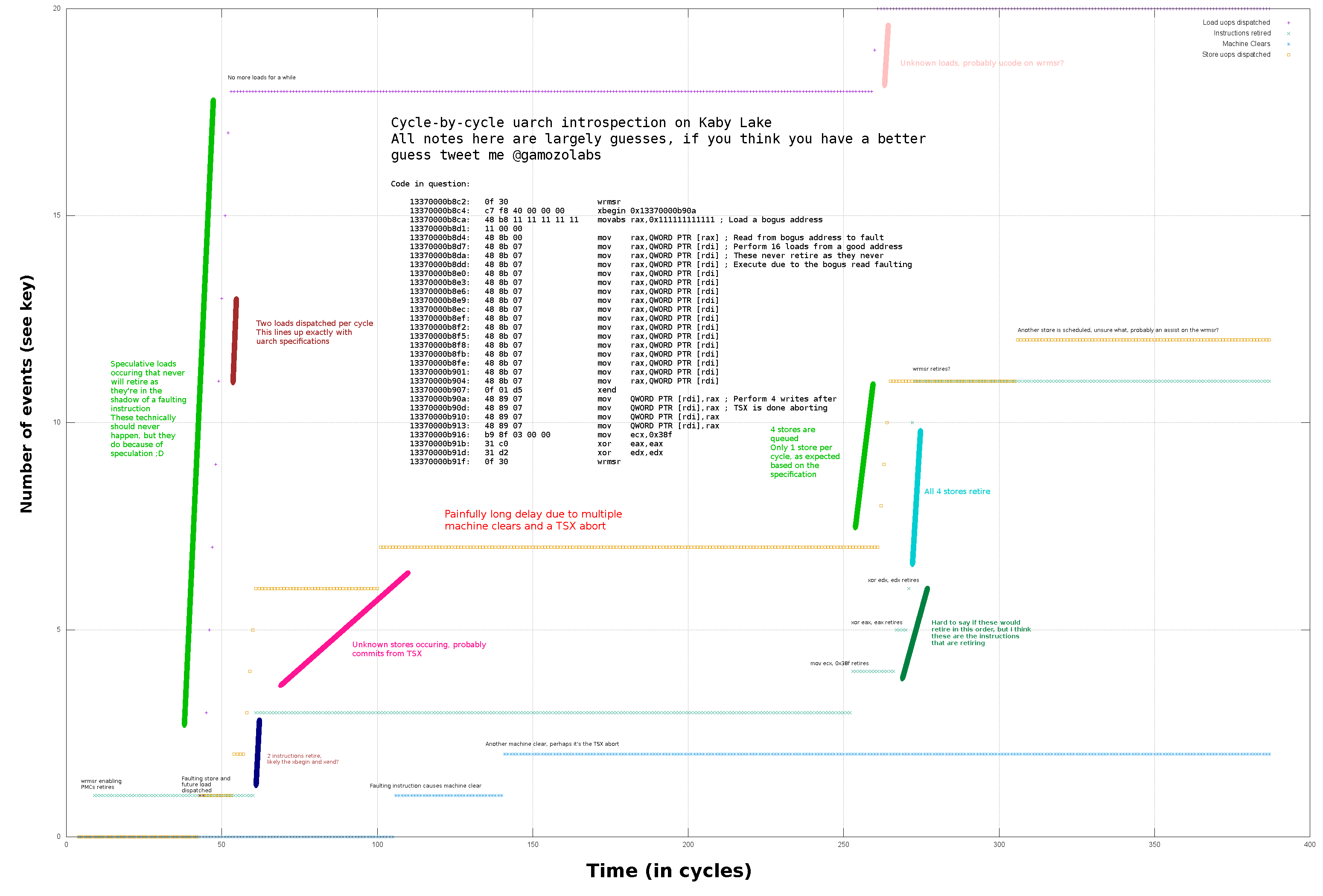
We’ll go a lot more into detail about what everything in this graph means later in the blog, but here’s a simple example of just some of the data we can collect:

_{Example cycle-by-cycle profiling of the Kaby Lake micro-architecture, warning: log-scale y-axis}

Agenda

This is a relatively long blog and will be split into 4 major sections.

• The gears that turn in your CPU: A high-level explanation of modern Intel micro-architectures
• Sushi Roll: The design of the low-noise research kernel
• Cycle-by-cycle micro-architectural introspection: A unique usage of performance counters to observe cycle-by-cycle micro-architectural behaviors
• Results: Putting the pieces together and making graphs of cool micro-architectural behavior

Why?

In the past year I’ve spent a decent amount of time doing CPU vulnerability research. I’ve written proof-of-concept exploits for nearly every CPU vulnerability, from many attacker perspectives (user leaking kernel, user/kernel leaking hypervisor, guest leaking other guest, etc). These exploits allowed us to provide developers and researchers with real-world attacks to verify mitigations.

CPU research happens to be an overlap of my two primary research interests: vulnerability research and high-performance kernel development. I joined Microsoft in the early winter of 2017 and this lined up pretty closely with the public release of the Meltdown and Spectre CPU attacks. As I didn’t yet have much on my plate, the idea was floated that I could look into some of the CPU vulnerabilities. I got pretty lucky with this timing, as I ended up really enjoying the work and ended up sinking most of my free time into it.

My workflow for research often starts with writing some custom tools for measuring and analysis of a given target. Whether the target is a web browser, PDF parser, remote attack surface, or a CPU, I’ve often found that the best thing you can do is just make something new. Try out some new attack surface, write a targeted fuzzer for a specific feature, etc. Doing something new doesn’t have to be better or more difficult than something that was done before, as often there are completely unexplored surfaces out there. My specialty is introspection. I find unique ways to measure behaviors, which then fuels the idea pool for code auditing or fuzzer development.

This leads to an interesting situation in CPU research… it’s largely blind. Lots of the current CPU research is done based on writing snippets of code and reviewing the overall side-effects of it (via cache timing, performance counters, etc). These overall side-effects may also include noise from other processor activity, from the OS task switching processes, other cores changing the MESI-state of cache lines, etc. I happened to already have a low-noise no-shared-memory research kernel that I developed for vectorized emulation on Xeon Phis! This lead to a really good starting point for throwing in some performance counters and measuring CPU behaviors… and the results were a bit better than expected.

TL;DR: I enjoy writing tools to measure things, so I wrote a tool to measure undefined CPU behavior.

The gears that turn in your CPU

Feel free to skip this section entirely if you’re familiar with modern processor architecture

Your modern Intel CPU is a fairly complex beast when you care about every technical detail, but lets look at it from a higher level. Here’s what the micro-architecture (uArch) looks like in a modern Intel Skylake processor.

_{Skylake uArch diagram, Diagram from WikiChip}

There are 3 main components: The front end, which converts complex x86 instructions into groups of micro-operations. The execution engine, which executes the micro-operations. And the memory subsystem, which makes sure that the processor is able to get streams of instructions and data.

Front End

The front end covers almost everything related to figuring out which micro-operations (uops) need to be dispatched to the execution engine in order to accomplish a task. The execution engine on a modern Intel processor does not directly execute x86 instructions, rather these instructions are converted to these micro-operations which are fixed in size and specific to the processor micro-architecture.

Instruction fetch and cache

There’s a lot that happens prior to the actual execution of an instruction. First, the memory containing the instruction is read into the L1 instruction cache, ideally brought in from the L2 cache as to minimize delay. At this point the instruction is still a macro-op (a variable-length x86 instruction), which is quite a pain to work with. The processor still doesn’t know how large the instruction is, so during pre-decode the processor will do an initial length decode to determine the instruction boundaries.

At this point the instruction has been chopped up and is ready for the instruction queue!

Instruction Queue and Macro Fusion

Instructions that come in for execution might be quite simple, and could potentially be “fused” into a complex operation. This stage is not publicly documented, but we know that a very common fusion is combining compare instructions with conditional branches. This allows a common instruction pattern like:

cmp rax, 5
jne .offset

To be combined into a single macro-op with the same semantics. This complex fused operation now only takes up one slot in many parts of the CPU pipeline, rather than two, freeing up more resources to other operations.

Decode

Instruction decode is where the x86 macro-ops get converted into micro-ops. These micro-ops vary heavily by uArch, and allow Intel to regularly change fundamentals in their processors without affecting backwards compatibility with the x86 architecture. There’s a lot of magic that happens in the decoder, but mostly what matters is that the variable-length macro-ops get converted into the fixed-length micro-ops. There are multiple ways that this conversion happens. Instructions might directly convert to uops, and this is the common path for most x86 instructions. However, some instructions, or even processor conditions, may cause something called microcode to get executed.

Microcode

Some instructions in x86 trigger microcode to be used. Microcode is effectively a tiny collection of uops which will be executed on certain conditions. Think of this like a C/C++ macro, where you can have a one-liner for something that expands to much more. When an operation does something that requires microcode, the microcode ROM is accessed and the uops it specifies are placed into the pipeline. These are often complex operations, like switching operating modes, reading/writing internal CPU registers, etc. This microcode ROM also gives Intel an opportunity to make changes to instruction behaviors entirely with a microcode patch.

uop Cache

There’s also a uop cache which allows previously decoded instructions to skip the entire pre-decode and decode process. Like standard memory caching, this provides a huge speedup and dramatically reduces bottlenecks in the front-end.

Allocation Queue

The allocation queue is responsible for holding a bunch of uops which need to be executed. These are then fed to the execution engine when the execution engine has resources available to execute them.

Execution engine

The execution engine does exactly what you would expect: it executes things. But at this stage your processor starts moving your instructions around to speed things up.

_{Things start to get a bit complex at this point, click for details!}

Renaming / Allocating / Retirement

Resources need to be allocated for certain operations. There are a lot more registers in the processor than the standard x86 registers. These registers are allocated out for temporary operations, and often mapped onto their corresponding x86 registers.

There are a lot of optimizations the CPU can do at this stage. It can eliminate register moves by aliasing registers (such that two x86 registers “point to” the same internal register). It can remove known zeroing instructions (like xor with self, or and with zero) from the pipeline, and just zero the registers directly. These optimizations are frequently improved each generation.

Finally, when instructions have completed successfully, they are retired. This retirement commits the internal micro-architectural state back out to the x86 architectural state. It’s also when memory operations become visible to other CPUs.

Re-ordering

uOP re-ordering is important to modern CPU performance. Future instructions which do not depend on the current instruction, could execute while waiting for the results of the current one.

For example:

mov rax, [rax]
add rbx, rcx

In this short example we see that we perform a 64-bit load from the address in rax and store it back into rax. Memory operations can be quite expensive, ranging from 4 cycles for a L1 cache hit, to 250 cycles and beyond for an off-processor memory access.

The processor is able to realize that the add rbx, rcx instruction does not need to “wait” for the result of the load, and can send off the add uop for execution while waiting for the load to complete.

This is where things can start to get weird. The processor starts to perform operations in a different order than what you told it to. The processor then holds the results and makes sure they “appear” to other cores in the correct order, as x86 is a strongly-ordered architecture. Other architectures like ARM are typically weakly-ordered, and it’s up to the developer to insert fences in the instruction stream to tell the processor the specific order operations need to complete in. This ordering is not an issue on a single core, but it may affect the way another core observes the memory transactions you perform.

For example:

Core 0 executes the following:

mov [shared_memory.pointer], rax ; Store the pointer in `rax` to shared memory
mov [shared_memory.owned],   0   ; Mark that we no longer own the shared memory

Core 1 executes the following:

.try_again:
    cmp [shared_memory.owned], 0 ; Check if someone owns this memory
    jne .try_again               ; Someone owns this memory, wait a bit longer

    mov rax, [shared_memory.pointer] ; Get the pointer
    mov rax, [rax]                   ; Read from the pointer

On x86 this is safe, as all aligned loads and stores are atomic, and are commit in a way that they appear in-order to all other processors. On something like ARM the owned value could be written to prior to pointer being written, allowing core 1 to use a stale/invalid pointer.

Execution Units

Finally we got to an easy part: the execution units. This is the silicon that is responsible for actually performing maths, loads, and stores. The core has multiple copies of this hardware logic for some of the common operations, which allows the same operation to be performed in parallel on separate data. For example, an add can be performed on 4 different execution units.

For things like loads, there are 2 load ports (port 2 and port 3), this allows 2 independent loads to be executed per cycle. Stores on the other hand, only have one port (port 4), and thus the core can only perform one store per cycle.

Memory subsystem

The memory subsystem on Intel is pretty complex, but we’re only going to go into the basics.

Caches

Caches are critical to modern CPU performance. RAM latency is so high (150-250 cycles) that a CPU is largely unusable without a cache. For example, if a modern x86 processor at 2.2 GHz had all caches disabled, it would never be able to execute more than ~15 million instructions per second. That’s as slow as an Intel 80486 from 1991.

When working on my first hypervisor I actually disabled all caching by mistake, and Windows took multiple hours to boot. It’s pretty incredible how important caches are.

For x86 there are typically 3 levels of cache: A level 1 cache, which is extremely fast, but small: 4 cycles latency. Followed by a level 2 cache, which is much larger, but still quite small: 14 cycles latency. Finally there’s the last-level-cache (LLC, typically the L3 cache), this is quite large, but has a higher latency: ~60 cycles.

The L1 and L2 caches are present in each core, however, the L3 cache is shared between multiple cores.

Translation Lookaside Buffers (TLBs)

In modern CPUs, applications almost never interface with physical memory directly. Rather they go through address translation to convert virtual addresses to physical addresses. This allows contiguous virtual memory regions to map to fragmented physical memory. Performing this translation requires 4 memory accesses (on 64-bit 4-level paging), and is quite expensive. Thus the CPU caches recently translated addresses such that it can skip this translation process during memory operations.

It is up to the OS to tell the CPU when to flush these TLBs via an invalidate page, invlpg instruction. If the OS doesn’t correctly invlpg memory when mappings change, it’s possible to use stale translation information.

Line fill buffers

While a load is pending, and not yet present in L1 cache, the data lives in a line fill buffer. The line fill buffers live between L2 cache and your L1 cache. When a memory access misses L1 cache, a line fill buffer entry is allocated, and once the load completes, the LFB is copied into the L1 cache and the LFB entry is discarded.

Store buffer

Store buffers are similar to line fill buffers. While waiting for resources to be available for a store to complete, it is placed into a store buffer. This allows for up to 56 stores (on Skylake) to be queued up, even if all other aspects of the memory subsystem are currently busy, or stores are not ready to be retired.

Further, loads which access memory will query the store buffers to potentially bypass the cache. If a read occurs on a recently stored location, the read could directly be filled from the store buffers. This is called store forwarding.

Load buffers

Similar to store buffers, load buffers are used for pending load uops. This sits between your execution units and L1 cache. This can hold up to 72 entries on Skylake.

CPU architecture summary and more info

That was a pretty high level introduction to many of the aspects of modern Intel CPU architecture. Every component of this diagram could have an entire blog written on it. Intel Manuals, WikiChip, Agner Fog’s CPU documentation, and many more, provide a more thorough documentation of Intel micro-architecture.

Sushi Roll

Sushi Roll is one of my favorite kernels! It wasn’t originally designed for CPU introspection, but it had some neat features which made it much more suitable for CPU research than my other kernels. We’ll talk a bit about why this kernel exists, and then talk about why it quickly became my go-to kernel for CPU research.

_{Kernel mascot: Squishble Sushi Roll}

A primer on Knights Landing

Sushi Roll was originally designed for my Vectorized Emulation work. Vectorized emulation was designed for the Intel Xeon Phi (Knights Landing), which is a pretty strange architecture. Even though it’s fully-featured traditional x86, standard software will “just work” on it, it is quite slow per individual thread. First of all, the clock rates are ~1.3 GHz, so there alone it’s about 2-3x slower than a “standard” x86 processor. Even further, it has fewer CPU resources for re-ordering and instruction decode. All-in-all the CPU is about 10x slower when running a single-threaded application compared to a “standard” 3 GHz modern Intel CPU. There’s also no L3 cache, so memory accesses can become much more expensive.

On top of these simple performance issues, there are more complex issues due to 4-way hyperthreading. Knights Landing was designed to be 4-way hyperthreaded (4 threads per core) to alleviate some of the performance losses of the limited instruction decode and caching. This allows threads to “block” on memory accesses while other threads with pending computations use the execution units. This 4-way hyperthreading, combined with 64-core processors, leads to 256 hardware threads showing up to your OS as cores.

Migrating processes and resources between these threads can be catastrophically slow. Standard shared-memory models also start to fall apart at this level of scaling (without specialized tuning). For example: If all 256 threads are hammering the same memory by performing an atomic increment (lock inc instruction), each individual increment will start to cost over 10,000 cycles! This is enough time for a single core on the Xeon Phi to do 640,000 single-precision floating point operations… just from a single increment! While most software treats atomics as “free locks”, they start to cause some serious cache-coherency pollution when scaled out this wide.

Obviously with some careful development you can mitigate these issues by decreasing the frequency of shared memory accesses. But perhaps we can develop a kernel that fundamentally disallows this behavior, preventing a developer from ever starting to go down the wrong path!

The original intent of Sushi Roll

Sushi Roll was designed from the start to be a massively parallel message-passing based kernel. The most notable feature of Sushi Roll is that there is no mutable shared memory allowed (a tiny exception made for the core IPC mechanism). This means that if you ever want to share information with another processor, you must pass that information via IPC. Shared immutable memory however, is allowed, as this doesn’t cause cache coherency traffic.

This design also meant that a lock never needed to be held, even atomic-level locks using the lock prefix. Rather than using locks, a specific core would own a hardware resource. For example, core #0 may own the network card, or a specific queue on the network card. Instead of requesting exclusive access to the NIC by obtaining a lock, you would send a message to core #0, indicating that you want to send a packet. All of the processing of these packets is done by the sender, thus the data is already formatted in a way that can be directly dropped into the NIC ring buffers. This made the owner of a hardware resource simply a mediator, reducing the latency to that resource.

While this makes the internals of the kernel a bit more complex, the programming model that a developer sees is still a standard send()/recv() model. By forcing message-passing, this ensured that all software written for this kernel could be scaled between multiple machines with no modification. On a single computer there is a fast, low-latency IPC mechanism that leverages some of the abilities to share memory (by transferring ownership of physical memory to the receiver). If the target for a message resided on another computer on the network, then the message would be serialized in a way that could be sent over the network. This complexity is yet again hidden from the developer, which allows for one program to be made that is scaled out without any extra effort.

No interrupts, no timers, no software threads, no processes

Sushi Roll follows a similar model to most of my other kernels. It has no interrupts, no timers, no software threads, and no processes. These are typically required for traditional operating systems, as to provide a user experience with multiple processes and users. However, my kernels are always designed for one purpose. This means the kernel boots up, and just does a given task on all cores (sometimes with one or two cores having a “special” responsibility).

By removing all of these external events, the CPU behaves a lot more deterministically. Sushi Roll goes the extra mile here, as it further reduces CPU noise by not having cores sharing memory and causing unexpected cache evictions or coherency traffic.

Soft Reboots

Similar to kexec on Linux, my kernels always support soft rebooting. This allows the old kernel (even a double faulted/corrupted kernel) to be replaced by a new kernel. This process takes about 200-300ms to tear down the old kernel, download the new one over PXE, and run the new one. This makes it feasible to have such a specialized kernel without processes, since I can just change the code of the kernel and boot up the new one in under a second. Rapid prototyping is crucial to fast development, and without this feature this kernel would be unusable.

Sushi Roll conclusion

Sushi Roll ended up being the perfect kernel for CPU introspection. It’s the lowest noise kernel I’ve ever developed, and it happened to also be my flagship kernel right as Spectre and Meltdown came out. By not having processes, threads, or interrupts, the CPU behaves much more deterministically than in a traditional OS.

Performance Counters

Before we get into how we got cycle-by-cycle micro-architectural data, we must learn a little bit about the performance monitoring available on Intel CPUs! This information can be explored in depth in the Intel System Developer Manual Volume 3b (note that the combined volume 3 manual doesn’t go into as much detail as the specific sub-volume manual).

Intel CPUs have a performance monitoring subsystem relying largely on a set of model-specific-registers (MSRs). These MSRs can be configured to track certain architectural events, typically by counting them. These counters are formally “performance monitoring counters”, often referred to as “performance counters” or PMCs.

These PMCs vary by micro-architecture. However, over time Intel has committed to offering a small subset of counters between multiple micro-architectures. These are called architectural performance counters. The version of these architectural performance counters are found in CPUID.0AH:EAX[7:0]. As of this writing there are 4 versions of architectural performance monitoring. The latest version provides a decent amount of generic information useful to general-purpose optimization. However, for a specific micro-architecture, the possibilities of performance events to track are almost limitless.

Basic usage of performance counters

To use the performance counters on Intel there are a few steps involved. First you must find a performance event you want to monitor. This information is found in per-micro-architecture tables found in the Intel Manual Volume 3b “Performance-Monitoring Events” chapter.

For example, here’s a very small selection of Skylake-specific performance events:

Intel performance counters largely rely on two banks of MSRs. The performance event selection MSRs, where the different events are programmed using the umask and event numbers from the table above. And the performance counter MSRs which hold the counts themselves.

The performance event selection MSRs (IA32_PERFEVTSELx) start at address 0x186 and span a contiguous MSR region. The layout of these event selection MSRs varies slightly by micro-architecture. The number of counters available varies by CPU and is dynamically checked by reading CPUID.0AH:EAX[15:8]. The performance counter MSRs (IA32_PMCx) start at address 0xc1 and also span a contiguous MSR region. The counters have an micro-architecture-specific number of bits they support, found in CPUID.0AH:EAX[23:16]. Reading and writing these MSRs is done via the rdmsr and wrmsr instructions respectively.

Typically modern Intel processors support 4 PMCs, and thus will have 4 event selection MSRs (0x186, 0x187, 0x188, and 0x189) and 4 counter MSRs (0xc1, 0xc2, 0xc3, and 0xc4). Most processors have 48-bit performance counters. It’s important to dynamically detect this information!

Here’s what the IA32_PERFEVTSELx MSR looks like for PMC version 3:

And that’s about it! Find the right event you want to track in your specific micro-architecture’s table, program it in one of the IA32_PERFEVTSELx registers with the correct event number and umask, set the USR and/or OS bits depending on what type of code you want to track, and set the E bit to enable it! Now the corresponding IA32_PMCx counter will be incrementing every time that event occurs!

Reading the PMC counts faster

Instead of performing a rdmsr instruction to read the IA32_PMCx values, instead a rdpmc instruction can be used. This instruction is optimized to be a little bit faster and supports a “fast read mode” if ecx[31] is set to 1. This is typically how you’d read the performance counters.

Performance Counters version 2

In the second version of performance counters, Intel added a bunch of new features.

Intel added some fixed performance counters (IA32_FIXED_CTR0 through IA32_FIXED_CTR2, starting at address 0x309) which are not programmable. These are configured by IA32_FIXED_CTR_CTRL at address 0x38d. Unlike normal PMCs, these cannot be programmed to count any event. Rather the controls for these only allows the selection of which CPU ring level they increment at (or none to disable it), and whether or not they trigger an interrupt on overflow. No other control is provided for these.

These are then enabled and disabled by:

The second version of performance counters also added 3 new MSRs that allow “bulk management” of performance counters. Rather than checking the status and enabling/disabling each performance counter individually, Intel added 3 global control MSRs. These are IA32_PERF_GLOBAL_CTRL (address 0x38f) which allows enabling and disabling performance counters in bulk. IA32_PERF_GLOBAL_STATUS (address 0x38e) which allows checking the overflow status of all performance counters in one rdmsr. And IA32_PERF_GLOBAL_OVF_CTRL (address 0x390) which allows for resetting the overflow status of all performance counters in one wrmsr. Since rdmsr and wrmsr are serializing instructions, these can be quite expensive and being able to reduce the amount of them is important!

Global control (simple, allows masking of individual counters from one MSR):

Status (tracks overflows of various counters, with a global condition changed tracker):

Status control (writing a 1 to any of these bits clears the corresponding bit in IA32_PERF_GLOBAL_STATUS):

Finally, Intel added 2 bits to the existing IA32_DEBUGCTL MSR (address 0x1d9). These 2 bits Freeze_LBR_On_PMI (bit 11) and Freeze_PerfMon_On_PMI (bit 12) allow freezing of last branch recording (LBR) and performance monitoring on performance monitor interrupts (often due to overflows). These are designed to reduce the measurement of the interrupt itself when an overflow condition occurs.

Performance Counters version 3

Performance counters version 3 was pretty simple. Intel added the ANY bit to IA32_PERFEVTSELx and IA32_FIXED_CTR_CTRL to allow tracking of performance events on any thread on a physical core. Further, the performance counters went from a fixed number of 2 counters, to a variable amount of counters. This resulted in more bits being added to the global status, overflow, and overflow control MSRs, to control the corresponding counters.

Performance Counters version 4

Performance counters version 4 is pretty complex in detail, but ultimately it’s fairly simple. Intel renamed some of the MSRs (for example IA32_PERF_GLOBAL_OVF_CTRL became IA32_PERF_GLOBAL_STATUS_RESET). Intel also added a new MSR IA32_PERF_GLOBAL_STATUS_SET (address 0x391) which instead of clearing the bits in IA32_PERF_GLOBAL_STATUS, allows for setting of the bits.

Further, the freezing behavior enabled by IA32_DEBUGCTL.Freeze_LBR_On_PMI and IA32_DEBUGCTL.Freeze_PerfMon_On_PMI was streamlined to have a single bit which tracks the “freeze” state of the PMCs, rather than clearing the corresponding bits in the IA32_PERF_GLOBAL_CTRL MSR. This change is awesome as it reduces the cost of freezing and unfreezing the performance monitoring unit (PMU), but it’s actually a breaking change from previous versions of performance counters.

Finally, they added a mechanism to allow sharing of performance counters between multiple users. This is not really relevant to anything we’re going to talk about, so we won’t go into details.

Conclusion

Performance counters started off pretty simple, but Intel added more and more features over time. However, these “new” features are critical to what we’re about to do next :)

Cycle-by-cycle micro-architectural sampling

Now that we’ve gotten some prerequisites out of the way, lets talk about the main course of this blog: A creative use of performance counters to get cycle-by-cycle micro-architectural information out of Intel CPUs!

It’s important to note that this technique is meant to assist in finding and learning things about CPUs. The data it generates is not particularly easy to interpret or work with, and there are many pitfalls to be aware of!

The Goal

Performance counters are incredibly useful in categorizing micro-architectural behavior on an Intel CPU. However, these counters are often used on a block or whole program entirely, and viewed as a single data point over the whole run. For example, one might use performance counters to track the number of times there’s a cache miss in their program under test. This will give a single number as an output, giving an indication of how many times the cache was missed, but it doesn’t help much in telling you when they occurred. By some binary searching (or creative use of counter overflows) you can get a general idea of when the event occurred, but I wanted more information.

More specifically, I wanted to view micro-architectural data on a graph, where the x-axis was in cycles. This would allow me to see (with cycle-level granularity) when certain events happened in the CPU.

The Idea

We’ve set a pretty lofty goal for ourselves. We effectively want to link two performance counters with each other. In this case we want to use an arbitrary performance counter for some event we’re interested in, and we want to link it to a performance counter tracking the number of cycles elapsed. However, there doesn’t seem to be a direct way to perform this linking.

We know that we can have multiple performance counters, so we can configure one to count a given event, and another to count cycles. However, in this case we’re not able to capture information at each cycle, as we have no way of reading these counters together. We also cannot stop the counters ourselves, as stopping the counters requires injecting a wrmsr instruction which cannot be done on an arbitrary cycle boundary, and definitely cannot be done during speculation.

But there’s a small little trick we can use. We can stop multiple performance counters at the same time by using the IA32_DEBUGCTL.Freeze_PerfMon_On_PMI feature. When a counter ends up overflowing, an interrupt occurs (if configured as such). When this overflow occurs, the freeze bit in IA32_PERF_GLOBAL_STATUS is set (version 4 PMCs specific feature), causing all performance counters to stop.

This means that if we can cause an overflow on each cycle boundary, we could potentially capture the time and the event we’re interested in at the same time. Doing this isn’t too difficult either, we can simply pre-program the performance counter value IA32_PMCx to N away from overflow. In our specific case, we’re dealing with a 48-bit performance counter. So in theory if we program PMC0 to count number of cycles, set the counter to 2^48 - N where N is >= 1, we can get an interrupt, and thus an “atomic” disabling of performance counters after N cycles.

If we set up a deterministic enough execution environment, we can run the same code over and over, while adjusting N to sample the code at a different cycle count.

This relies on a lot of assumptions. We’re assuming that the freeze bit ends up disabling both performance counters at the same time (“atomically”), we’re assuming we can cause this interrupt on an arbitrary cycle boundary (even during multi-cycle instructions), and we also are assuming that we can execute code in a clean enough environment where we can do multiple runs measuring different cycle offsets.

So… lets try it!

The Implementation

A simple pseudo-code implementation of this sampling method looks as such:

/// Number of times we want to sample each data point. This allows us to look
/// for the minimum, maximum, and average values. This also gives us a way to
/// verify that the environment we're in is deterministic and the results are
/// sane. If minimum == maximum over many samples, it's safe to say we have a
/// very clear picture of what is happening.
const NUM_SAMPLES: u64 = 1000;

/// Maximum number of cycles to sample on the x-axis. This limits the sampling
/// space.
const MAX_CYCLES: u64 = 1000;

// Program the APIC to map the performance counter overflow interrupts to a
// stub assembly routine which simply `iret`s out
configure_pmc_interrupts_in_apic();

// Configure performance counters to freeze on interrupts
perf_freeze_on_overflow();

// Iterate through each performance counter we want to gather data on
for perf_counter in performance_counters_of_interest {
    // Disable and reset all performance counters individually
    // Clearing their counts to 0, and clearing their event select MSRs to 0
    disable_all_perf_counters();

    // Disable performance counters globally by setting IA32_PERF_GLOBAL_CTRL
    // to 0
    disable_perf_globally();

    // Enable a performance counter (lets say PMC0) to track the `perf_counter`
    // we're interested in. Note that this doesn't start the counter yet, as we
    // still have the counters globally disabled.
    enable_perf_counter(perf_counter);

    // Go through each number of samples we want to collect for this performance
    // counter... for each cycle offset.
    for _ in 0..NUM_SAMPLES {
        // Go through each cycle we want to observe
        for cycle_offset in 1..=MAX_CYCLES {
            // Clear out the performance counter values: IA32_PMCx fields
            clear_perf_counters();

            // Program fixed counter #1 (un-halted cycle counter) to trigger
            // an interrupt on overflow. This will cause an interrupt, which
            // will then cause a freeze of all PMCs.
            program_fixed1_interrupt_on_overflow();

            // Program the fixed counter #1 (un-halted cycle counter) to
            // `cycles` prior to overflowing
            set_fixed1_value((1 << 48) - cycle_offset);

            // Do some pre-test environment setup. This is important to make
            // sure we can sample the code under test multiple times and get
            // the same result. Here is where you'd be flushing cache lines,
            // maybe doing a `wbinvd`, etc.
            set_up_environment();

            // Enable both the fixed #1 cycle counter and the PMC0 performance
            // counter (tracking the stat we're interested in) at the same time,
            // by using IA32_PERF_GLOBAL_CTRL. This is serializing so you don't
            // have to worry about re-ordering across this boundary.
            enable_perf_globally();

            asm!(r#"

                asm
                under
                test
                here

            "# :::: "volatile");

            // Clear IA32_PERF_GLOBAL_CTRL to 0 to stop counters
            disable_perf_globally();

            // If fixed PMC #1 has not overflowed, then we didn't capture
            // relevant data. This only can happen if we tried to sample a
            // cycle which happens after the assembly under test executed.
            if fixed1_pmc_overflowed() == false {
                continue;
            }

            // At this point we can do whatever we want as the performance
            // counters have been turned off by the interrupt and we should have
            // relevant data in both :)

            // Get the count from fixed #1 PMC. It's important that we grab this
            // as interrupts are not deterministic, and thus it's possible we
            // "overshoot" the target
            let fixed1_count = read_fixed1_counter();

            // Add the distance-from-overflow we initially programmed into the
            // fixed #1 counter, with the current value of the fixed #1 counter
            // to get the total number of cycles which have elapsed during
            // our example.
            let total_cycles = cycle_offset + fixed1_count;

            // Read the actual count from the performance counter we were using.
            // In this case we were using PMC #0 to track our event of interest.
            let value = read_pmc0();

            // Somehow log that performance counter `perf_counter` had a value
            // `value` `total_cycles` into execution
            log_result(perf_counter, value, total_cycles);
        }
    }
}

Simple results

So? Does it work? Let’s try with a simple example of code that just does a few “nops” by adjusting the stack a few times:

add rsp, 8
sub rsp, 8
add rsp, 8
sub rsp, 8

So how do we read this graph? Well, the x-axis is simple. It’s the time, in cycles, of execution. The y-axis is the number of events (which varies based on the key). In this case we’re only graphing the number of instructions retired (successfully executed).

So does this look right? Hmmm…. we ran 4 instructions, why did we see 8 retire?

Well in this case there’s a little bit of “extra” noise introduced by the harnessing around the code under test. Let’s zoom out from our code and look at what actually executes during our test:

; Right before test, we end up enabling all performance counters at once by
; writing 0x2_0000_000f to IA32_PERF_GLOBAL_CTRL. This enables all 4
; programmable counters at the same time as enabling fixed PMC #1 (cycle count)
00000000  B98F030000        mov ecx,0x38f ; IA32_PERF_GLOBAL_CTRL
00000005  B80F000000        mov eax,0xf
0000000A  BA02000000        mov edx,0x2
0000000F  0F30              wrmsr

; Here's our code under test :D
00000011  4883C408          add rsp,byte +0x8
00000015  4883EC08          sub rsp,byte +0x8
00000019  4883C408          add rsp,byte +0x8
0000001D  4883EC08          sub rsp,byte +0x8

; And finally we disable all counters by setting IA32_PERF_GLOBAL_CTRL to 0
00000021  B98F030000        mov ecx,0x38f
00000026  31C0              xor eax,eax
00000028  31D2              xor edx,edx
0000002A  0F30              wrmsr

So if we take another look at the graph, we see there are 8 instructions that retired. The very first instruction we see retire (at cycle=11), is actually the wrmsr we used to enable the counters. This makes sense, at some point prior to retirement of the wrmsr instruction the counters must be enabled internally somewhere in the CPU. So we actually get to see this instruction retire!

Then we see 7 more instructions retire to give us a total of 8… hmm. Well, we have 4 of our add and sub mix that we executed, so that brings us down to 3 more remaining “unknown” instructions.

These 3 remaining instructions are explained by the code which disables the performance counter after our test code has executed. We have 1 mov, and 2 xor instructions which retire prior to the wrmsr which disables the counters. It makes sense that we never see the final wrmsr retire as the counters will be turned off in the CPU prior to the wrmsr instruction retiring!

Wala! It all makes sense. We now have a great view into what the CPU did in terms of retirement for this code in question. Everything we saw lined up with what actually executed, always good to see.

A bit more advanced result

Lets add a few more performance counters to track. In this case lets track the number of instructions retired, as well as the number of micro-ops dispatched to port 4 (the store port). This will give us the number of stores which occurred during test.

Code to test (just a few writes to the stack):

; Right before test, we end up enabling all performance counters at once by
; writing 0x2_0000_000f to IA32_PERF_GLOBAL_CTRL. This enables all 4
; programmable counters at the same time as enabling fixed PMC #1 (cycle count)
00000000  B98F030000        mov ecx,0x38f
00000005  B80F000000        mov eax,0xf
0000000A  BA02000000        mov edx,0x2
0000000F  0F30              wrmsr

00000011  4883EC08          sub rsp,byte +0x8
00000015  48C7042400000000  mov qword [rsp],0x0
0000001D  4883C408          add rsp,byte +0x8
00000021  4883EC08          sub rsp,byte +0x8
00000025  48C7042400000000  mov qword [rsp],0x0
0000002D  4883C408          add rsp,byte +0x8

; And finally we disable all counters by setting IA32_PERF_GLOBAL_CTRL to 0
00000031  B98F030000        mov ecx,0x38f
00000036  31C0              xor eax,eax
00000038  31D2              xor edx,edx
0000003A  0F30              wrmsr

This one is fun. We simply make room on the stack (sub rsp), write a 0 to the stack (mov [rsp]), and then restore the stack (add rsp), and then do it all again one more time.

Here we added another plot to the graph, Port 4, which is the store uOP port on the CPU. We also track the number of instructions retired, as we did in the first example. Here we can see instructions retired matches what we would expect. We see 10 retirements, 1 from the first wrmsr enabling the performance counters, 6 from our own code under test, and 3 more from the disabling of the performance counters.

This time we’re able to see where the stores occur, and indeed, 2 stores do occur. We see a store happen at cycle=28 and cycle=29. Interestingly we see the stores are back-to-back, even though there’s a bit of code between them. We’re probably observing some re-ordering! Later in the graph (cycle=39), we observe that 4 instructions get retired in a single cycle! How cool is that?!

How deep can we go?

Using the exact same store example from above, we can enable even more performance counters. This gives us an even more detailed view of different parts of the micro-architectural state.

In this case we’re tracking all uOP port activity, machine clears (when the CPU resets itself after speculation), offcore requests (when messages get sent offcore, typically to access physical memory), instructions retired, and branches retired. In theory we can measure any possible performance counter available on our micro-architecture on a time domain. This gives us the ability to see almost anything that is happening on the CPU!

Noise…

In all of the examples we’ve looked at, none of the data points have visible error bars. In these graphs the error bars represent the minimum value, mean value, and maximum value observed for a given data point. Since we’re running the same code over and over, and sampling it at different execution times, it’s very possible for “random” noise to interfere with results. Let’s look at a bit more noisy example:

; Right before test, we end up enabling all performance counters at once by
; writing 0x2_0000_000f to IA32_PERF_GLOBAL_CTRL. This enables all 4
; programmable counters at the same time as enabling fixed PMC #1 (cycle count)
00000000  B98F030000        mov ecx,0x38f
00000005  B80F000000        mov eax,0xf
0000000A  BA02000000        mov edx,0x2
0000000F  0F30              wrmsr

00000011  48C7042500000000  mov qword [0x0],0x0
         -00000000
0000001D  48C7042500000000  mov qword [0x0],0x0
         -00000000
00000029  48C7042500000000  mov qword [0x0],0x0
         -00000000
00000035  48C7042500000000  mov qword [0x0],0x0
         -00000000

; And finally we disable all counters by setting IA32_PERF_GLOBAL_CTRL to 0
00000041  B98F030000        mov ecx,0x38f
00000046  31C0              xor eax,eax
00000048  31D2              xor edx,edx
0000004A  0F30              wrmsr

Here we’re just going to write to NULL 4 times. This might sound bad, but in this example I mapped NULL in as normal write-back memory. Nothing crazy, just treat it as a valid address.

But here are the results:

Hmmm… we have error bars! We see the stores always get dispatched at the same time. This makes sense, we’re always doing the same thing. But we see that some of the instructions have some variance in where they retire. For example, at cycle=38 we see that sometimes at this point 2 instructions have been retired, other times 4 have been retired, but on average a little over 3 instructions have been retired at this point. This tells us that the CPU isn’t always deterministic in this environment.

These results can get a bit more complex to interpret, but it’s still relevant data nevertheless. Changing the code under test, cleaning up to the environment to be more determinsitic, etc, can often improve the quality and visibility of the data.

Does it work with speculation?

Damn right it does! That was the whole point!

Let’s cause a fault, perform some loads behind it, and see if we can see the loads get issued even though the entire section of code is discarded.

    // Start a TSX section, think of this as a `try {` block
    xbegin 2f

    // Read from -1, causing a fault
    mov rax, [-1]

    // Here's some loads shadowing the faulting load. These
    // should never occur, as the instruction above causes
    // an exeception and thus execution should "jump" to the label `2:`

    .rept 32
        // Repeated load 32 times
        mov rbx, [0]
    .endr

    // End the TSX section, think of this as a `}` closing the
    // `try` block
    xend

2:
    // Here is where execution goes if the TSX section had
    // an exception, and thus where execution will flow

Both ports 2 and port 3 are load ports. We see both of them taking turns handling loads (1 load per cycle each, with 2 ports, 2 loads per cycle total). Here we can see many different loads get dispatched, even though very few instructions actually retire. What we’re viewing here is the micro-architecture performing speculation! Neat!

More data?

I could go on and on graphing different CPU behaviors! There’s so much cool stuff to explore out there. However, this blog has already gotten longer than I wanted, so I’ll stop here. Maybe I’ll make future small blogs about certain interesting behaviors!

Conclusion

This technique of measuring performance counters on a time-domain seems to work quite well. You have to be very careful with noise, but with careful interpretation of the data, this technique provides the highest level of visibility into the Intel micro-architecture that I’ve ever seen!

This tool is incredibly useful for validating hypothesises about behaviors of various Intel micro-architectures. By running multiple experiments on different behaviors, a more macro-level model can be derived about the inner workings of the CPU. This could lead to learning new optimization techniques, finding new CPU vulnerabilities, and just in general having fun learning how things work!

Source?

Update: 8/19/2019

This kernel has too many sensitive features that I do not want to make public at this time…

However, it seems there’s a lot of interest in this tech, so I will try to live stream soon adding this functionality to my already-open-source kernel Orange Slice!

Twitter

Follow me at @gamozolabs on Twitter if you want notifications when new blogs come up. I also do random one-off posts for cool data that doesn’t warrant an entire blog!

Let me know if you like this mini-blog format! It takes a lot less time than a whole blog, but I think will still have interesting content!

Prereqs

You should probably read the Introduction to Vectorized Emulation blog!

Or perhaps watch the talk I gave at RECON 2019

Summary

I spent this weekend working on a JIT for my IL (FalkIL, or fail). I thought this would be a cool opportunity to make a mini-blog describing how I currently handle conditional branches in vectorized emulation.

This is one of the most complex parts of vectorized emulation, and has a lot of depth. But today we’re going to go into a simple merging example. What I call the “auto-merge”. I call it an auto-merge because it doesn’t require any static analysis of potential merging points. The instructions that get emit simply allow for auto re-merging of divergent VMs. It’s really simple, but pretty nifty. We have to perform this logic on every branch.

FalkIL Example

Here’s an example of what FalkIL looks like:

JIT

Here’s what the JIT for the above IL example looks like:

Ooof… that exploded a bit. Let’s dive in!

JIT Calling Convention

Before we can go into what the JIT is doing, we have to understand the calling convention we use. It’s important to note that this calling convention is custom, and follows no standard convention.

Kmask Registers

Kmask registers are the bitmasks provided to us in hardware to mask off certain operations. Since we’re always executing instructions even if some VMs have been disabled, we must always honor using kmasks.

Intel provides us with 8 kmask registers. k0 through k7. k0 is hardcoded in hardware to all ones (no masking). Thus, we’re not able to use this for general purpose masking.

Online VM mask

Since at any given time we might be performing operations with VMs disabled, we need to have one kmask register always dedicated to holding the mask of VMs that are actively running. Since k1 is the first general purpose kmask we can use, that’s exactly what we pick. Any bit which is clear in k1 (VM is disabled), must not have its state modified. Thus you’ll see k1 is used as a merging mask for almost every single vectorized operation we do.

By using the k1 mask in every instruction, we preseve the lanes of vector registers which are disabled. This provides near-zero-cost preservation of disabled VM states, such that we don’t have to save/restore massive ZMM registers during divergence.

This mask must also be honored during scalar code that emulates complex vectorized operations (for example divs, which have no vectorized instruction).

“Following” VM mask

At some points during emulation we run into situations where VMs have to get disabled. For example, some VMs might take a true branch, and others might take the false (or “else”) side of a branch. In this case we need to make a decision (very quickly) about which VM to follow. To do this, we have a VM which we mark as the “following” VM. We store this “following” VM mask in k7. This always contains a single bit, and it’s the bit of the VM which we will always follow when we have to make divergence decisions.

The VM we are “following” must always be active, and thus (k7 & k1) != 0 must always be true! This k7 mask only has to be updated when we enter the JIT, thus the computation of which VM to “follow” may be complex as it will not be a common expense. While the JIT is executing, this k7 mask will never have to be updated unless the VM we are following causes a fault (at which point a new VM to follow will be computed).

Kmask Register Summary

Here’s the complete state of kmask register allocation during JIT

K0    - Hardcoded in hardware to all ones
K1    - Bitmask indicating "active/online" VMs
K2-K6 - Scratch kmask registers
K7    - "Following" VM mask

ZMM registers

The 512-bit ZMM registers are where we store most of our active contextual data. There are only 2 special case ZMM registers which we reserve.

“Following” VM index vector

Following in the same suit of the “Following VM mask”, mentioned above, we also store the index for the “following” VM in all 8 64-bit lanes of zmm30. This is needed to make decisions about which VM to follow. At certain points we will need to see which VM’s “agree with” the VM we are following, and thus we need a way to quickly broadcast out the following VMs values to all components of a vector.

By holding the index (effectively the bit index of the following VM mask) in all lanes of the zmm30 vector, we can perform a single vpermq instruction to broadcast the following VM’s value to all lanes in a vector.

Similar to the VM mask, this only needs to be computed when the JIT is entered and when faults occur. This means this can be a more expensive operation to fill this register up, as it stays the same for the entirity of a JIT execution (until a JIT/VM exit).

Why this is important

Lets say:

zmm31 contains [10, 11, 12, 13, 14, 15, 16, 17]

zmm30 contains [3, 3, 3, 3, 3, 3, 3, 3]

The CPU then executes vpermq zmm0, zmm30, zmm31

zmm0 now contains [13, 13, 13, 13, 13, 13, 13, 13]… the 3rd VM’s value in zmm31 broadcast to all lanes of zmm0

Effectively vpermq uses the indicies in its second operand to select values from the third operand.

“Desired target” vector

We allocate one other ZMM register (zmm31) to hold the block identifiers for where each lane “wants” to execute. What this means is that when divergence occurs, zmm31 will have the corresponding lane updated to where the VM that diverged “wanted” to go. VMs which were disabled thus can be analyzed to see where they “wanted” to go, but instead they got disabled :(

ZMM Register Summary

Here’s the complete state of ZMM register allocation during JIT

Zmm0-Zmm3  - Scratch registers for internal JIT use
Zmm4-Zmm29 - Used for IL register allocation
Zmm30      - Index of the VM we are following broadcast to all 8 quadwords
Zmm31      - Branch targets for each VM, indicates where all VMs want to execute

General purpose registers

These are fairly simple. It’s a lot more complex when we talk about memory accesses and such, but we already talked about that in the MMU blog!

When ignoring the MMU, there are only 2 GPRs that we have a special use for…

Constant storage database

On the Knights Landing Xeon Phi (the CPU I develop vectorized emulation for), there is a huge bottleneck on the front-end and instruction decode. This means that loading a constant into a vector register by loading it into a GPR mov, then moving it into the lowest-order lane of a vector vmovq, and then broadcasting it vpbroadcastq, is actually a lot more expensive than just loading that value from memory.

To enable this, we need a database which just holds constants. During the JIT, constants are allocated from this table (just appending to a list, while deduping shared constants). This table is then pointed to by r11 during JIT. During the JIT we can load a constant into all active lanes of a VM by doing a single vpbroadcastq zmm, kmask, qword [r11+OFFSET] instruction.

While this might not be ideal for normal Xeon processors, this is actually something that I have benchmarked, and on the Xeon Phi, it’s much faster to use the constant storage database.

Target registers

At the end of the day we’re emulating some other architecture. We hold all target architecture registers in memory pointed to by r12. It’s that simple. Most of the time we hold these in IL registers and thus aren’t incurring the cost of accessing memory.

GPR summary

r11 - Points to constant storage database (big vector of quadword constants)
r12 - Points to target architecture registers

Phew

Okay, now we know what register states look like when executing in JIT!

Conditional branches

Now we can get to the meat of this mini-blog! How conditional branches work using auto-merging! We’re going to go through instruction-by-instruction from the JIT graph we showed above.

Here’s the specific code in question for a conditional branch:

Well that looks awfully complex… but it’s really not. It’s quite magical!

The comparison

First, the comparision is performed on all lanes. Remember, ZMM registers hold 8 separate 64-bit values. We perform a 64-bit unsigned comparison on all 8 components, and store the results into k2. This means that k2 will hold a bitmask with the “true” results set to 1, and the “false” results set to 0. We also use a kmask k1 here, which means we only perform the comparison on VMs which are currently active. As a result of this instruction, k2 has the corresponding bits set to 1 for VMs which were actively executing at the time, and also resulted in a “true” value from their comparisons.

In this case the 0x1 immediate to the vpcmpuq instruction indicates that this is a “less than” comparison.

vpcmpq/vpcmpuq immediate

Note that the immediate value provided to vpcmpq and the unsigned variant vpcmpuq determines the type of the comparison:

The comparison inversion

Next, we invert the comparison operation to get the bits set for active VMs which want to go to the “false” path. This instruction is pretty neat.

kandnw performs a bitwise negation of the second operand, and then ands with the third operand. This then is stored into the first operand. Since we have k2 as the second operand (the result of the comparison) this gets negated. This then gets anded with k1 (the third operand) to mask off VMs which are not actively executing. The result is that k3 now contains the inverted result from the comparison, but we keep “offline” VMs still masked off.

In C/C++ this is simply: k3 = (~k2) & k1

The branch target vector

Now we start constructing zmm0… this is going to hold the “labels” for the targets each active lane wants to go to. Think of these “labels” as just a unique identifier for the target block they are branching to. In this case we use the constant storage database (pointed to by r11) to load up the target labels. We first load the “true target” labels into zmm0 by using the k2 kmask, the “true” kmask. After this, we merge the “false target” labels into zmm0 using k3, the “false/inverted” kmask.

After these 2 instructions execute, zmm0 now holds the target “labels” based on their corresponding comparison results. zmm0 now tells us where the currently executing VMs “want to” branch to.

The merge into master

Now we merge the target branches for the active VMs which were just computed (zmm0), into the master target register (zmm31). Since VMs can be disabled via divergence, zmm31 holds the “master” copy of where all VMs want to go (including ones which have been masked off and are “waiting” to execute a certain target).

zmm31 now holds the target labels for every single lane with the updated results of this comparison!

Broadcasting the target

Now that we have zmm31 containing all of the branch targets, we now have to pick the one we are going to follow. To do this, we want a vector which contains the broadcasted target label of the VM we are following. As mentioned in the JIT calling convention section, zmm30 contains the index of the VM we are following in all 8 lanes.

Example

Lets say for example we are following VM #4 (zero-indexed).

zmm30 contains [4, 4, 4, 4, 4, 4, 4, 4]

zmm31 contains [block_0, block_0, block_1, block_1, block_2, block_2, block_2, block_2]

After the vpermq instruction we now have zmm1 containing [block_2, block_2, block_2, block_2, block_2, block_2, block_2, block_2].

Effectively, zmm1 will contain the block label for the target that the VM we are following is going to go to. This is ultimately the block we will be jumping to!

Auto-merging

This is where the magic happens. zmm31 contains where all the VMs “want to execute”, and zmm1 from the above instruction contains where we are actually going to execute. Thus, we compute a new k1 (active VM kmask) based on equality between zmm31 and zmm1.

Or in more simple terms… if a VM that was previously disabled was waiting to execute the block we’re about to go execute… bring it back online!

Doin’ the branch

Now we’re at the end. k2 still holds the true targets. We and this with k7 (the “following” VM mask) to figure out if the VM we are following is going to take the branch or not.

We then need to make this result “actionable” by getting it into the eflags x86 register such that we can conditionally branch. This is done with a simple kortestw instruction of k2 with itself. This will cause the zero flag to get set in eflags if k2 is equal to zero.

Once this is done, we can do a jnz instruction (same as jne), causing us to jump to the true target path if the k2 value is non-zero (if the VM we’re following is taking the true path). Otherwise we fall through to the “false” path (or potentially branch to it if it’s not directly following this block).

Update

After a little nap, I realized that I could save 2 instructions during the conditional branch. I knew something was a little off as I’ve written similar code before and I never needed an inverse mask.

Here we’ll note that we removed 2 instructions. We no longer compute the inverse mask. Instead, we initially store the false target block labels into zmm31 using the online mask (k1). This temporarly marks that “all online VMs want to take the false target”. Then, using the k2 mask (true targets), merge over zmm31 with the true target block labels.

Simple! We remove the inverse mask computation kandnw, and the use of the zmm0 temporary and merge directly into zmm31. But the effect is exactly the same as the previous version.

Not quite sure why I thought the inverse mask was needed, but it goes to show that a little bit of rest goes a long way!

Due to instruction decode pressure on the Xeon Phi (2 instructions decoded per cycle), this change is a minimum 1 cycle improvement. Further, it’s a reduction of 8 bytes of code per conditional branch, which reduces L1i pressure. This is likely in the single digit percentages for overall JIT speedup, as conditional branches are everywhere!

Fin

And that’s it! That’s currently how I handle auto-merging during conditional branches in vectorized emulation as of today! This code is often changed and this is probably not its final form. There might be a simpler way to achieve this (fewer instructions, or lower latency instructions)… but progress always happens over time :)

It’s important to note that this auto-merging isn’t perfect, and most cases will result in VMs hanging, but this is an extremely low cost way to bring VMs online dynamically in even the tightest loops. More macro-scale merging can be done with smarter static-analysis and control flow decisions.

I hope this was a fun read! Let me know if you want more of these mini-blogs.

_{Frequencies of observed values over time from load ports. Here we’re seeing the processor internally performing a microcode-assisted page table walk to update accessed and dirty bits. Only one load was performed by the user, these are all “invisible” loads done behind the scenes}

Twitter

Follow me at @gamozolabs on Twitter if you want notifications when new blogs come up. I often will post data and graphs from data as it comes in and I learn!

Foreward

First of all, I’d like to say that I’m super excited to write up this blog. This is an idea I’ve had for over a year and I only recently got to working on. The initial implementation and proof-of-concept of this idea was actually implemented live on my Twitch! This proof-of-concept went from nothing at all to a fully-working-as-predicted implementation in just about 3 hours! Not only did the implementation go much smoother than expected, the results are by far higher resolution and signal-to-noise than I expected!

This blog is fairly technical, and thus I highly recommend that you read my previous blog on Sushi Roll, my CPU research kernel where this technique was implemented. In the Sushi Roll blog I go a little bit more into the high-level details of Intel micro-architecture and it’s a great introduction to the topic if you’re not familiar.

_{Recording of the stream where we implemented this idea as a proof-of-concept. Click for the YouTube video!}

Summary

We’re going to go into a unique technique for observing and sequencing all load port traffic on Intel processors. By using a CPU vulnerability from the MDS set of vulnerabilities, specifically multi-architectural load port data sampling (MLPDS, CVE-2018-12127), we are able to observe values which fly by on the load ports. Since (to my knowledge) all loads must end up going through load ports, regardless of requestor, origin, or caching, this means in theory, all contents of loads ever performed can be observed. By using a creative scanning technique we’re able to not only view “random” loads as they go by, but sequence loads to determine the ordering and timing of them.

We’ll go through some examples demonstrating that this technique can be used to view all loads as they are performed on a cycle-by-cycle basis. We’ll look into an interesting case of the micro-architecture updating accessed and dirty bits using a microcode assist. These are invisible loads dispatched on the CPU on behalf of the user when a page is accessed for the first time.

Why

As you may be familiar, x86 is quite a complex architecture with many nooks and crannies. As time has passed it has only gotten more complex, leading to fewer known behaviors of the inner workings. There are many instructions with complex microcode invocations which access memory as were seen through my work on Sushi Roll. This led to me being curious as to what is actually going on with load ports during some of these operations.

_{Intel CPU traffic on load ports (ports 2 and 3) and store ports (port 4) during a traditional memory write}

_{Intel CPU traffic on load ports (ports 2 and 3) and store ports (port 4) during the same memory write as above, but this time where the page table entries need an accessed/dirty bit update}

Beyond just directly invoked microcode due to instructions being executed, microcode also gets executed on the processor during “microcode assists”. These operations, while often undocumented, are referenced a few times throughout Intel manuals. Specifically in the Intel Optimization Manual there are references to microcode assists during accessed and dirty bit updates. Further, there is a restriction on TSX sections such that they may abort when accessed and dirty bits need to be updated. These microcode assists are fascinating to me, as while I have no evidence for it, I suspect they may be subject to different levels of permissions and validations compared to traditional operations. Whenever I see code executing on a processor as a side-effect to user operations, all I think is: “here be dragons”.

A playground for CPU bugs

When I start auditing a target, the first thing that I try to do is get introspection into what is going on. If the target is an obscure device then I’ll likely try to find some bug that allows me to image the entire device, and load it up in an emulator. If it’s some source code I have that is partial, then I’ll try to get some sort of mocking of the external calls it’s making and implement them as I come by them. Once I have the target running on my terms, and not the terms of some locked down device or environment, then I’ll start trying to learn as much about it as possible…

This is no different from what I did when I got into CPU research. Starting with when Meltdown and Spectre came out I started to be the go-to person for writing PoCs for CPU bugs. I developed a few custom OSes early on that were just designed to give a pass/fail indicator if a CPU bug were able to be exploited in a given environment. This was critical in helping test the mitigations that went in place for each CPU bug as they were reported, as testing if these mitigations worked is a surprisingly hard problem.

This led to me having some cleanly made OS-level CPU exploits written up. The custom OS proved to be a great way to test the mitigations, especially as the signal was much higher compared to a traditional OS. In fact, the signal was almost just a bit too strong…

When in a custom operating system it’s a lot easier to play around with weird behaviors of the CPU, without worrying about it affecting the system’s stability. I can easily turn off interrupts, overwrite exception handlers with specialized ones, change MSRs to weird CPU states, and so on. This led to me ending up with almost a playground for CPU vulnerability testing with some pretty standard primitives.

As the number of primitives I had grew, I was able to PoC out a new CPU bug in typically under a day. But then I had to wonder… what would happen if I tried to get the most information out of the processor as possible.

Sushi Roll

And that was the starting of Sushi Roll, my CPU research kernel. I have a whole blog about the Sushi Roll research kernel, and I strongly recommend you read it! Effectively Sushi Roll is a custom kernel with message passing between cores rather than memory sharing. This means that each core has a complete copy of the kernel with no shared accesses. For attacks which need to observe the faintest signal in memory behaviors, this lead to a great amount of isolation.

When looking for a behavior you already understand on a processor, it’s pretty easy to get a signal. But, when doing initial CPU research into the unknowns and undefined behavior, getting this signal out takes every advantage as you can get. Thus in this low-noise CPU research environment, even the faintest leak would cause a pretty large disruption in determinism, which would likely show up as a measurable result earlier than traditional blind CPU research would allow.

Performance Counter Monitoring

In Sushi Roll I implemented a creative technique for monitoring the values in performance counters along with time-stamping them in cycles. Some of the performance counters in Intel processors count things like the number of micro-ops dispatched to each of the execution units on the core. Some of these counters increase during speculation, and with this data and time-stamping I was able to get some of the first-ever insights into what processor behavior was actually occurring during speculation!

_{Example cycle-by-cycle profiling of the Kaby Lake micro-architecture, warning: log-scale y-axis}

Being able to collect this sort of data immediately made unexpected CPU behaviors easier to catalog, measure, and eventually make determinstic. The more understanding we can get of the internals of the CPU, the better!

The Ultimate Goal

The ultimate goal of my CPU research is to understand so thoroughly how the Intel micro-architecture works that I can predict it with emulation models. This means that I would like to run code through an emulated environment and it would tell me exactly how many internal CPU resources would be used, which lines from caches and buffers would be evicted and what contents they would hold. There’s something beautiful to me to understanding something so well that you can predict how it will behave. And so the journey begins…

Past Progress

So far with the work in Sushi Roll we’ve been able to observe how the CPU dispatches uops during specific portions of code. This allows us to see which CPU resources are used to fulfill certain requests, and thus can provide us with a rough outline of what is happening. With simple CPU operations this is often all we need, as there are only so many ways to perform a certain operation, the complete picture can usually be drawn just from guessing “how they might have done it”. However, when more complex operations are involved, all of that goes out the window.

When reading through Intel manuals I saw many references to microcode assists. These are “situations” in your processor which may require microcode to be dispatched to execution units to perform some complex-ish logic. These are typically edge cases which don’t occur frequently enough for the processor to worry about handling them in hardware, rather just needing to detect them and cause some assist code to run. We know of one microcode assist which is relatively easy to trigger, updating the accessed and dirty bits in the page tables.

Accessed and dirty bits

In the Intel page table (and honestly most other architectures) there’s a concept of accessed and dirty bits. These bits indicate whether or not a page has ever been translated (accessed), or if it has been written to (dirtied). On Intel it’s a little strange as there is only a dirty bit on the final page table entry. However, the accessed bits are present on each level of the page table during the walk. I’m quite familiar with these bits from my work with hypervisor-based fuzzing as it allows high performance differential resetting of VMs by simply walking the page tables and restoring pages that were dirtied to their original state of a snapshot.

But this leads to an curiosity… what is the mechanic responsible for setting these bits? Does the internal page table silicon set these during a page table walk? Are they set after the fact? Are they atomically set? Are they set during speculation or faulting loads?

From Intel manuals and some restrictions with TSX it’s pretty obvious that accessed and dirty bits are a bit of an anomaly. TSX regions will abort when memory is touched that does not have the respective accessed or dirty bits set. Which is strange, why would this be a limitation of the processor?

_{Accessed and dirty bits causing TSX aborts from the Intel® 64 and IA-32 architectures optimization reference manual}

… weird huh? Testing it out yields exactly what the manual says. If I write up some sample code which accesses memory which doesn’t have the respective accessed or dirty bits set, it aborts every time!

What’s next?

So now we have an ability to view what operation types are being performed on the processor. However this doesn’t tell us a huge amount of information. What we would really benefit from would be knowing the data contents that are being operated on. We can pretty easily log the data we are fetching in our own code, but that won’t give us access to the internal loads that happen as side effects on the processor, nor would it tell us about the contents of loads which happen during speculation.

Surely there’s no way to view all loads which happen on the processor right? Almost anything during speculation is a pain to observe, and even if we could observe the data it’d be quite noisy.

Or maybe there is a way…

… a way?

Fortunately there may indeed be a way! A while back I found a CPU vulnerability which allowed for random values to be sampled off of the load ports. While this vulnerability is initially thought to only allow for random values to be sampled from the load ports, perhaps we can get a bit more creative about leaking…

Multi-Architectural Load Port Data Sampling (MLPDS)

Multi-architectural load port data sampling sounds like an overly complex name, but it’s actually quite simple in the end. It’s a set of CPU flaws in Intel processors which allow a user to potentially get access to stale data recently transferred through load ports. This was actually a bug that I reported to Intel a while back and they ended up finding a few similar issues with different instruction combinations, this is ultimately what comprises MLPDS.

Description of MLPDS from Intel’s MDS DeepDive

The specific bug that I found was initially called “cache line split” or “cache line split load” and it’s exactly what you might expect. When a data access straddles a cache line (multi-byte load containing some bytes on one cache line and the remaining bytes on another). Cache lines are 64-bytes in size so any multi-byte memory access to an address with the bottom 6 bits set would cause this behavior. These accesses must also cause a fault or an assist, but by using TSX it’s pretty easy to get whatever behavior you would like.

This bug is largely an issue when hyper-threading is enabled as this allows a sibling thread to be executing protected/privileged code while another thread uses this attack to observe recently loaded data.

I found this bug when working on early PoCs of L1TF when we were assessing the impact it had. In my L1TF PoC (which was using random virtual addresses each attempt) I ended up disabling the page table modification. This ultimately is the root requirement for L1TF to work, and to my surprise, I was still seeing a signal. I initially thought it was some sort of CPU bug leaking registers as the value I was leaking was never actually read in my code. It turns out what I ended up observing was the hypervisor itself context switching my VM. What I was leaking was the contents of the registers as they were loaded during the context switch!

Unfortunately MLPDS has a really complex PoC…

mov rax, [-1]

After this instruction executes and it faults or aborts, the contents of rax during a small speculative window will potentially contain stale data from load ports. That’s all it takes!

From this point it’s just some trickery to get the 64-bit value leaked during the speculative window!

It’s all too random

Okay, so MLPDS allows us to sample a “random” value which was recently loaded on the load ports. This is a great start as we could probably run this attack over and over and see what data is observed on a sample piece of code. Using hyper-threading for this attack will be ideal because we can have one thread running some sample code in an infinite loop, while the other code observes the values seen on the load port.

An MLPDS exploit

Since there isn’t yet a public exploit for MLPDS, especially with the data rates we’re going to use here, I’m just going to go over the high-level details and not show how it’s implemented under the hood.

For this MLPDS exploit I use a couple different primitives. One is a pretty basic exploit which simply attempts to leak the raw contents of the value which was leaked. This value that we leak is always 64-bits, but we can chose to only leak a few of the bytes from it (or even bit-level granularity). There’s a performance increase for the fewer bytes that we leak as it decreases the number of cache lines we need to prime-and-probe each attempt.

There’s also another exploit type that I use that allows me to look for a specific value in memory, which turns the leak from a multi-byte leak to just a boolean “was value/wasn’t value”. This is the highest performance version due to how little information has to be leaked past the speculative window.

All of these leaks will leak a specific value from a single speculative run. For example if we were to leak a 64-bit value, the 64-bit value will be from one MLPDS exploit and one speculative window. Getting an entire 64-bit value out during a single speculative window is a surprisingly hard problem, and I’m going to keep that as my own special sauce for a while. Compared to many public CPU leak exploits, this attack does not loop multiple times using masks to slowly reveal a value, it will get revealed from a single attempt. This is critical to us as otherwise we wouldn’t be able to observe values which are loaded once.

Here’s some of the leak rate numbers for the current version of MLPDS that I’m using:

It’s important to note that the known 64-bit value search is much faster than all of the others. We’ll make some good use of this later!

Test

Let’s try out a simple MLPDS attack on a small piece of code which loops forever fetching 2 values from memory.

mov  rax, 0x12345678f00dfeed
mov [0x1000], rax

mov  rax, 0x1337133713371337
mov [0x1008], rax

2:
    mov rax, [0x1000]
    mov rax, [0x1008]
    jmp 2b

This code should in theory just causes two loads. One of a value 0x12345678f00dfeed and another of a value 0x1337133713371337. Lets spin this up on a hardware thread and have the sibling thread perform MLPDS in a loop! We’ll use our 64-bit any value MLPDS attack and just histogram all of the different values we observe get leaked.

Sampling done:
    0x12345678f00dfeed : 100532
    0x1337133713371337 : 99217

Viola! Here we see the two different secret values on the attacking thread, at a pretty much comparable frequency.

Cool… so now we have a technique that will allow us to see the contents of all loads on load ports, but randomly sampled only. Let’s take a look at the weird behaviors during accessed bit updates by clearing the accessed bit on the final level page tables every loop in the same code above.

Sampling done:
    0x0000000000000008 : 559
    0x0000000000000009 : 2316
    0x000000000000000a : 142
    0x000000000000000e : 251
    0x0000000000000010 : 825
    0x0000000000000100 : 19
    0x0000000000000200 : 3
    0x0000000000010006 : 438
    0x000000002cc8c000 : 3796
    0x000000002cc8c027 : 225
    0x000000002cc8d000 : 112
    0x000000002cc8d027 : 57
    0x000000002cc8e000 : 1
    0x000000002cc8e027 : 35
    0x00000000ffff8bc2 : 302
    0x00002da0ea6a5b78 : 1456
    0x00002da0ea6a5ba0 : 2034
    0x0000700dfeed0000 : 246
    0x0000700dfeed0008 : 5081
    0x0000930000000000 : 4097
    0x00209b0000000000 : 15101
    0x1337133713371337 : 2028
    0xfc91ee000008b7a6 : 677
    0xffff8bc2fc91b7c4 : 2658
    0xffff8bc2fc9209ed : 4565
    0xffff8bc2fc934019 : 2

Whoa! That’s a lot more values than we saw before. They weren’t from just the two values we’re loading in a loop, to many other values. Strangely the 0x1234... value is missing as well. Interesting. Well since we know these are accessed bit updates, perhaps some of these are entries from the page table walk. Let’s look at the addresses of the page table entry we’re hitting.

CR3   0x630000
PML4E 0x2cc8e007
PDPE  0x2cc8d007
PDE   0x2cc8c007
PTE   0x13370003

Oh! How cool is that!? In the loads we’re leaking we see the raw page table entries with various versions of the accessed and dirty bits set! Here are the loads which stand out to me:

Leaked values:

    0x000000002cc8c000 : 3796                                                   
    0x000000002cc8c027 : 225                                                    
    0x000000002cc8d000 : 112                                                    
    0x000000002cc8d027 : 57                                                     
    0x000000002cc8e000 : 1                                                      
    0x000000002cc8e027 : 35 

Actual page table entries for the page we're accessing:

CR3   0x630000                                                                  
PML4E 0x2cc8e007                                                                
PDPE  0x2cc8d007                                                                
PDE   0x2cc8c007                                                                
PTE   0x13370003

The entries are being observed as 0x...27 as the 0x20 bit is the accessed bit for page table entries.

Other notable entries are 0x0000930000000000 and 0x00209b0000000000 which look like the GDT entries for the code and data segments. 0x0000700dfeed0000 and 0x0000700dfeed0008 which are the 2 virtual addresses I’m accessing the un-accessed memory from. Who knows about the rest of the values? Probably some stack addresses in there…

So clearly as we expected, the processor is dispatching uops which are performing a page table walk. Sadly we have no idea what the order of this walk is, maybe we can find a creative technique for sequencing these loads…

Sequencing the Loads

Sequencing the loads that we are leaking with MLPDS is going to be critical to getting meaningful information. Without knowing the ordering of the loads we simply know contents of loads. Which is a pretty awesome amount of information, I’m definitely not complaining… but come on, it’s not perfect!

But perhaps we can limit the timing of our attack to a specific window, and infer ordering based on that. If we can find some trigger point where we can synchronize time between the attacker thread and the thread with secrets, we could change the delay between this synchronization and the leak attempt. By scanning this leak we should hopefully get to see a cycle-by-cycle view of observed values.

A trigger point

We can perform an MLPDS attack on a delay, however we need a reference point to delay from. I’ll steal the oscilloscope terminology of a trigger, or a reference location to synchronize with. Similar to an oscilloscope this trigger will synchronize our on the time domain each time we attempt.

The easiest trigger we can use works only in an environment where we control both the leaking and secret threads, but in our case we have that control.

What we can do is simply have semaphores at each stage of the leak. We’ll have 2 hardware threads running with the following logic:

1. (Thread A running) (Thread B paused)
2. (Thread A) Prepare to do a CPU attack, request thread B execute code
3. (Thread A) Delay for a fixed amount of cycles with a spin loop
4. (Thread B) Execute sample code
5. (Thread A) At some “random” point during Thread B executing sample code, perform MLPDS attack to leak a value
6. (Thread B) Complete sample code execution, wait for thread A to request another execution
7. (Thread A) Log the observed value and the number of cycles in the delay loop
8. goto 0 and do this many times until significant data is collected

Uncontrolled target code

If needed a trigger could be set on a “known value” at some point during execution if target code is not controllable. For example, if you’re attacking a kernel, you could identify a magic value or known user pointer which gets accessed close to the code under test. An MLPDS attack can be performed until this magic value is seen, then a delay can start, and another attack can be used to leak a value. This allows an uncontrolled target code to be sampled in a similar way. If the trigger “misses” it’s fine, just try again in another loop.

Did it work?

So we put all of these things together, but does it actually work? Lets try our 2 load example, and we’ll make sure they depend on each other to ensure they don’t get re-ordered by the processor.

Prep code:

core::ptr::write_volatile(vaddr as *mut u64, 0x12341337cafefeed);              
core::ptr::write_volatile((vaddr as *mut u64).offset(1), 0x1337133713371337);  

Test code:

let ptr = core::ptr::read_volatile(vaddr as *mut usize);
core::ptr::read_volatile((vaddr as usize + (ptr & 0x8)) as *mut usize);

In this code we set up 2 dependant loads. One which reads a value, and then another which masks the value to get the 8th bit, which is used as an offset to a subsequent access. Since the values are constants, we know that the second access will always access at offset 8, thus we expect to see a load of 0x1234... followed by 0x1337....

Graphing the data

To graph the data we have collected, we want to collect the frequencies each value was seen for every cycle offset. We’ll plot these with an x axis in cycles, and a y axis in frequency the value was observed at that cycle count. Then we’ll overlay multiple graphs for the different values we’ve seen. Let’s check it out in our simple case test code!

_{Sequenced leak example data}

Here we also introduce a normal distribution best-fit for each value type, and a vertical line through the mean frequency-weighted value.

And look at that! We see the first access (in light blue) indicating that the value 0x12341337cafefeed was read, and slightly after we see (in orange) the value 0x1337133713371337 was read! Exactly what we would have expected. How cool is that!? There’s some other noise on here from the testing harness, but they’re pretty easy to ignore in this case.

A real-data case

Let’s put it all together and take a look at what a load looks like on pages which have not yet been marked as accessed.

_{Frequencies of observed values over time from load ports. Here we’re seeing the processor internally performing a microcode-assisted page table walk to update accessed and dirty bits. Only one load was performed by the user, these are all “invisible” loads done behind the scenes}

Hmmm, this is a bit too noisy. Let’s re-collect the data but this time only look at the page table entry values and the value contained on the page we’re accessing.

Here are the page table entries for the memory we’re accessing in our example:

CR3   0x630000
PML4E 0x2cc7c007
PDPE  0x2cc7b007
PDE   0x2cc7a007
PTE   0x13370003
Data  0x12341337cafefeed

We’re going to reset all page table entries to their non-dirty, non-accessed states, invalidate the TLB for the page via invlpg, and then read from the memory once. This will cause all accessed bits to be updated in the page tables! Here’s what we get…

_{Annotated ucode-assist page walk as observed with this technique}

Here it’s hard to say why we see the 3rd and 4th levels of the page table get hit, as well as the page contents, prior to the accessed bit updates. Perhaps the processor tries the access first, and when it realizes the accessed bits are not set it goes through and sets them all. We can see fairly clearly that after this page data is read ~300 cycles in, that it performs a page-by-page walk through each level. Presumably this is where the processor is reading the original values from pages, oring in the accessed bit, and moving to the next level!

Speeding it up

So far using our 64-bit MLPDS leak we can get about 8,000 leaks per second. This is a decent data rate, but when we’re wanting to sample data and draw statistical significance, more is always better. For each different value we want to log, and for each cycle count, we likely want about ~100 points of data. So lets assume we want to sample 10 values over a 1000 cycle range, and we’ll likely want 1 million data points. This means we’ll need about 2 minutes worth of runtime to collect this data.

Luckily, there’s a relatively simple technique we can use to speed up the data rates. Instead of using the full arbitrary 64-bit leak for the whole test, we can use the arbitrary leak early on to determine the values of interest. We just want to use the arbitrary leak for long enough to determine the values which we know are accessed during our test case.

Once we know the values we actually want to leak, we can switch to using our known-value leak which allows for about 6 million leaks per second. Since this can only look for one value at a time, we’ll also have to cycle through the values in our “known value” list, but the speedup is still worth it until the known value list gets incredibly large.

With this technique, collecting the 1 million data points for something with 5-6 values to sample only takes about a second. A speedup of two orders of magnitude! This is the technique that I’m currently using, although I have a fallback to arbitrary value mode if needed for some future use.

Conclusion

We introduced an interesting technique for monitoring Intel load port traffic cycle-by-cycle and demonstrated that it can be used to get meaningful data to learn how Intel micro-architecture works. While there is much more for us to poke around in, this was a simple example to show this technique!

Future

There is so much more I want to do with this work. First of all, this will just be polished in my toolbox and used for future CPU research. It’ll just be a good go-to tool for when I need a little bit more introspection. But, I’m sure as time goes on I’ll come up with new interesting things to monitor. Getting logging of store-port activity would be useful such that we could see the other side of memory transactions.

As with anything I do, performance is always an opportunity for improvement. Getting a higher-fidelity MLPDS exploit, potentially with higher throughput, would always help make collecting data easier. I’ve also got some fun ideas for filtering this data to remove “deterministic noise”. Since we’re attacking from a sibling hyperthread I suspect we’d see some deterministic sliding and interleaving of core usage. If I could isolate these down and remove the noise that’d help a lot.

I hope you enjoyed this blog! See you next time!

Summary

Welcome to fuzz week 2020! This week (July 13th - July 17th) I’ll be streaming every day going through some of the very basics of fuzzing all the way to cutting edge research. I want to use this time to talk about some things related to fuzzing, particularly when it comes to benchmarking and comparing fuzzers with each other.

Schedule

Ha. There’s really no schedule, there is no script, there is no plan, but here’s a rough outline of what I want to cover.

I will be streaming on my Twitch channel at approximately 14:00 PST. But things aren’t really going to be on a strict schedule.

My Twitter is probably the best source of information for when things are about to start.

Everything will be recorded and uploaded to my YouTube.

July 13th

The very basics of fuzzing. We’ll write our own fuzzer and tweak it to improve it. We’ll probably start by writing it in Python, and eventually talk about the performance ramifications and the basics of scaling fuzzers by using threads or multiple processes. We’ll also compare our newly written fuzzer against AFL and see where AFL outperforms it, and also where AFL has some blind spots.

July 14th

Here we’ll cover code coverage. We might get to this sooner, who knows. But we’re going to write our own tooling to gather code coverage information such that we can see not only how easy it is to set up, but how flexible coverage information can be while still proving quite useful!

July 15th-17th

Here we’ll focus mainly on the advanced aspects of fuzzing. While this sounds complex, fuzzing really hasn’t become that complex yet, so follow along! We’ll go through some of the more deep performance properties of fuzzing, mainly focused around snapshot fuzzing.

Once we’ve discussed some basics of performance and snapshot fuzzing, we’ll start talking about the meaningfulness of comparing fuzzers. Namely, the difficulties in comparing fuzzers when they may involve different concepts of what a crash, coverage, or input are. We’ll look at some existing examples of papers which compare fuzzers, and see how well they actually prove their point.

Biases

I think it’s important when doing something like this, to make it clear what my existing biases are. I’ve got a few.

• I think existing fuzzers have some major performance problems and struggle to scale. I consider this to be a high priority as general performance improvements to fuzzing harnesses makes both generic fuzzers (eg. AFL, context-unaware fuzzers) and hand-crafted (targeted) fuzzers better.
• I don’t think outperforming AFL is impressive. AFL is impressive because it’s got an easy-to-use workflow, which makes it accessible to many different users, broadening the amount of targets it has been used against.
• I don’t really thinking comparing fuzzers is reasonable.
• I think it is very easy to over-fit a fuzzer to small programs, or add unrealistic amounts of information extraction from a target under test, in a way that the concepts are not generally applicable to many targets that exceed basic parsers. I think this is where a lot of current research falls.

But… that’s mainly the point of this week. To either find out my biases are wildly incorrect, or to maybe demonstrate why I have some of the biases. So, how will I address some of these (in order of prior bullets)?

• I’ll compare some of my fuzzers against AFL. We’ll see if we can outperform AFL in terms of raw fuzz cases performed, as well as the results (coverage and crashes).
• I’ll try to demonstrate that a basic fuzzer with 1/100th the amount of code of AFL is capable of getting much better results, and that it’s really not that hard to write.
• I’ll propose some techniques that can be used to compare fuzzers, and go through my own personal process of evaluating fuzzers. I’m not trying to get papers, or funding, or anything. I don’t really have an interest in making things look comparatively better. If they perform differently, but have different use cases, I’d rather understand those cases and apply them specifically rather than have a one-shoe-fits-all solution.
• I’ll go through some instrumentation that I’ve historically added to my fuzzers which give them massive result and coverage boosts, but consume so much information that they cannot meaningfully scale past tiny pieces of code. I’ll go through when these things may actually be useful, as sometimes isolating components is viable. I’ll also go through some existing papers and see what sorts of results are being claimed, and if they actually have general applicability.

Winging it

It’s important to note, nothing here is scheduled. Things may go much faster, slower, or just never happen. That’s the beauty of research. I may be very wrong with some of my biases, and we’ll hopefully correct those. I love being wrong.

I’ve maybe thought of having some fuzzing figureheads pop on the stream for random discussions/conversations/interviews. If this is something that sounds interesting to you, reach out and we can maybe organize it!

Sound fun?

See you there :)

Foreward

This blog is a bit weird, this is actually a message I posted in response to a fuzzbench issue, but honestly, I think it warranted a blog, even if it’s a bit unpolished!

You can find the discussion at fuzzbench issue tracker #654

Social

I’ve been streaming a lot more regularly on my Twitch! I’ve developed hypervisors for fuzzing, mutators, emulators, and just done a lot of fun fuzzing work on stream. Come on by!

Follow me at @gamozolabs on Twitter if you want notifications when new blogs come up. I often will post data and graphs from data as it comes in and I learn!

The blog

Hello again Today!

So, I’d like to address a few things that I’ve thought of a bit more over time and want to emphasize.

Visualizations, and what I’m often looking for in data

When it comes to visualizations, I don’t really mind much which graphs are displayed by default, linear vs logscale, time-based or per-case-based, but they should both be toggleable in the default. I’m not web dev, but having an interactive graph would be pretty nice, allowing for turning on and off of certain lines, zooming in and out, and changing scales/axes. But, I think we’re in agreement here. I personally believe that logscale should be default, and I don’t see how it’s anything but better, unless you only care about seeing where things “flatten out”. But in that case, it’s just as visible in logscale, you just have to be logscale aware.

Here’s an example of typically what I graph when I’m running and tuning a fuzzer. I’m using doing side-by-side comparisons of small fuzzer tweaks, to my prior best runs, and plotting both on a time domain and a fuzz case domain. I’ve included the linear-scale plots just for comparison with the way we currently do things, but I personally never use linear scale as I just find it to be worse in all aspects.

By using a linear scale, we’re unable to see anything about what happens in the fuzzer in the first ~20 min or so. We just see a vertical line. In the log scale we see a lot more which is happening. This graph is comparing a fuzzer which does rand() % 20 rounds of mutation (medium corruption), versus rand % 5 rounds of the same corruption (low corruption). We can see that early on medium corruption has much better properties, as it explores more aggressively. But there’s actually a point where they cross, and this is likely the point where the corruption becomes too great on average in the medium corruption, and ends up “ruining” previously good inputs, dramatically reducing the frequency we see good cases. It’s important to note, that since the medium corruption is a superset of low corruption (eg, there’s a chance to do low corruption), both graphs would eventually converge to the exact same value.

There’s just so much information in this graph that stands out to me. I see that something about medium corruption performs well in the first ~100 seconds. There’s a really good lead at the early few seconds, and it tapers off throughout. This gives me feedback on maybe when and where I should use this level of corruption.

Further, since I have both a fuzz case graph and a time graph, I can see that medium corruption early on actually has better performance than low corruption. Once again, this makes sense, the more corruption, the more likely you are to make a more invalid input which is parsed more shallow. But from the coverage over case, I see that this isn’t a long term thing and eventually the performance seems to converge between the two. It’s important to note, the intersection point of the two lines varies by quite a bit in both the case domain and the time domain. This tells me that even though I just changed the mutator, it has affected the performance, likely due to the depth of the average input in the corpus, really neat!

Example analysis conclusion

I see that medium corruption in this case is giving me about 10x speedup in time-to-same-coverage, and also some performance benefits early on. I should adopt a dynamic corruption model which tunes this corruption amount maybe against time, or ideally, some other metric I could extract from the target or stats. I see that long-term, the low corruption starts to win, and for something that I’d run for a week, I’d much rather run the low corruption.

Even though this program is very simple, these graphs could pretty arbitrary be stretched out to different time axis. If fuzzbench picks a deadline, for example, 1000 seconds, we would never know this about the fuzzer performance. I think this is likely what many fuzzers are now being tuned to, as the benchmarks often are 12/24/72 hour increments. Fuzzers often get some extra blips even deeper in the runs, and it’s really hard to estimate if these crosses would ever occur.

The case for cases

I personally extract most information from graphs which are plotted against number of fuzz cases rather than time. By doing benchmarks in a time domain, you factor in the performance of the fuzzer. This is this ground truth, and what really matters at the end of the day with complete products. But it’s not the ground truth for fuzzers in development. For example, if I wanted to prototype a new mutation strategy for AFL, I would be forced to do it in C, avoid inefficient copies, avoid mallocs, etc. I effectively have to make sure my mutator is at-or-better than existing AFL mutator performance to use benchmarks like this.

When you do development on fuzz cases, you can start to inspect the efficiency of the fuzzer in terms of quality of cases produced. I could prototype a mutator in python for all I care, and see if it performs better than the stock AFL mutators. This allows me to cut corners and spend 1 day trying out a mutator, rather than 1 month making a mutator and then doing complex optimizations to make it work. During early stages of development, I would expect a developer to understand the ramifications of making it faster, and to have a ballpark idea of where it could be if the O(n^3) logic was turned into O(log n), and whether it’s possible.

Often times, the first pass of an attempt is going to be crude, and for no reason other than laziness (and not in a negative way)! There’s a time and a place to polish and optimize a technique, and it’s important that there can be information learned from very preliminary results. Most performance in standard feedback mechanisms and mutation strategies can be solved with a little bit of engineering, and most developers should be able to gauge the best-case big-O for their strategy, even if that’s not the algorithmic complexity of their initial implementation.

Yep, looking at coverage over cases adds nuance, but I think we can handle it. Given most fuzzing tools, especially initial passes, are already so un-optimized, I’m really not worried about any performance differences in AFL/libfuzzer/etc when it comes to single-core performance.

Scaling

Scaling of performance is really missing from fuzzbench. At every company I’ve worked at, big and small, even for the most simple targets we’re fuzzing we’re running at least ~50-100 cores. I presume (I don’t know for sure) that fuzzbench is comparing single core performance. That’s great, it’s a useful stat and one I often control for, as single-core, coverage/case is often controlled for both scaling and performance, leading to great introspection into the raw logic of the fuzzer.

However, in reality, the scaling of these tools is critical for actual use. If AFL is 20% faster single-core, that’ll likely make it show up at the top of fuzzbench, given relative parity of mutation strategies. That’s great, the performance takes engineering effort and should not be undervalued. In fact, most of my research is focused around making fuzzers fast, I’ve got multiple fuzzers that can handle 10s of billions of fuzz cases per second on a single machine. It’s a lot of work to make these tools scale, much more so than single-core performance, which is often algorithmic fixes.

If AFL is 20% faster single-core, but bottlenecks on fork(), or write(), and thus only scales to 20-30 cores (often where I see AFL really fall apart, on medium size targets, 5-10 cores for small targets). But something like libfuzzer manages things in memory and can scale linearly with as many cores as you throw it, libfuzzer is going to blow away any 20% performance gains seen single-core.

This information is very hard to benchmark. Well, not hard, but costly. Effectively, I’d like to see benchmarks of fuzzers scaled to ~16 cores on a single server, and ~128 cores distributed across at least 4 servers. This benchmarks. A. the possibility the fuzzer can scale in the first place, if it can’t that’s a big hit to real-world usability. B. the possibility it can scale across servers (often, over the network). Things like AFL-over-SMB would have brutal scaling properties here. C. the scalability properties between cores on the same server, and how they transfer over the network.

I find it very unlikely that these fuzzers being benchmarked even remotely have similar scaling properties. AFL struggles to scale even on a single server, even in persistent mode, due to the heavy use of syscalls and blocking IPC every fuzz case (signal(), read(), write(), per case IIRC, ~3-4 syscalls).

Scaling also puts a lot of pressure on infeasible fuzzing strategies proposed in papers. We’ve all seen them, the high-introspection techniques which extract memory, register, taint state from a small program and promise great results. I don’t disagree with the results, the more information you extract, pretty much directly correlates to an increase in coverage/case. But, eventually the data load gets very hard to share between cores, queue between servers, and even just process.

Measuring symbolic

Measuring symbolic was brought up a few times, as it would definitely have a much better coverage/case than a traditional fuzzer. But this nuance can easily be handled by looking at both coverage/case and coverage/time graphs. Learning what works well algorithmicly should drive our engineering efforts to solve problems. While symbolic may have huge performance issues, it’s very likely, that many of the parts of it (eg. taint tracking) can be approximated with lossy algorithms and data capturing, and it’s more about learning where it has strengths and weaknesses. Many of the analyses I’ve done on symbolic largely lead me to vectorized emulation, which allows for highly-compressed, approximated taint tracking, while still getting near-native (or even better) execution speeds.

The case against monolithic fuzzers

Learning what works is important to figure out where to invest our engineering time. Given the quality of code in fuzzing right now (often very poor), there’s a lot of things that I’d hate to see us rule out because our current methodologies do not support them. I really care about my reset times of fuzz cases, (often: the fork() costs), as well as determinism. In a fully deterministic environment, with fast resets, a lot of approximate strategies can be used. Trying to approximate where bytes came from in an input, flipping the bytes because you have a branch target which is interesting, and then smashing those bytes in can give good information about the relation of those bytes to the input. Hell, with fast resets and forking, you can do partial fuzzing where you fork() and snapshot multiple times during a fuzz case, and you can progressively fuzz “from” different points in the parser. This works especially well for protocols where you can snapshot at each packet boundary.

These sorts of techniques and analyses don’t really work when we have monolithic fuzzers. The performance of existing fuzzers is often quite poor (AFL fork(), etc), or does not support partial execution (persistent modes, libfuzzer, etc). This leads to us not being able to even research these techniques. As we keep bolting things onto existing fuzzers and treating them like big blobs, we’ll get further and further from being able to learn the isolated properties of fuzzers and find the best places to apply certain strategies.

Why I don’t care much about fuzzer performance for benchmarking

Reset speed

AFL fork() bottlenecks for me often around 10-20k execs/sec on a single core, and about 40-50k on the whole system, even with 96C/192T systems. This is largely due to just getting stuck on kernel allocations and locks. Spinning up processes is expensive, and largely out of our control. AFL allows access of the local system and kernel to the fuzz case, thus cases are not deterministic, nor are they isolated (in the case of fuzzing something with lock files). This requires using another abstraction layer like docker, which adds more overhead to the equation. My hypervisors that I use for fuzzing can reset a Windows VM 1 million times per second on a single core, and scale linearly with cores, while being deterministic. Why does this matter? Well, we’re comparing tooling which isn’t even remotely hitting the capabilities of the CPUs, rather they’re bottlenecking on the kernel. These are solvable problems, and thus, as a consumer of good ideas but not tooling, I’m interested in what works well. I can make it go fast myself.

Determinism

Most fuzzers that we work with now are not deterministic. You cannot expect instruction-for-instruction determinism between cases. This makes it a lot harder to use complex fuzzing strategies which may rely on the results of a prior execution being identical to a future one. This is largely an engineering problem, and can be solved in both system-level and app-level targets.

Mutation performance

The performance of mutators is often not what it can be. For example, honggfuzz used (now fixed, cheers!) temporary allocations during multiple passes. During its mangle_MemSwap it made a copy of the chunk that was to be swapped, performing 3 memcpys and using a temporary allocation. This logic was able to be implemented using a single memcpy and without a dynamic allocation. This is not a criticism of honggfuzz, but more of an important note of how development often occurs. Early prototyping, success, and rare revisiting of what can be changed. What’s my point here? Well, the mutation strategies in many fuzzers may introduce timing properties that are not fundamentally required to have identical behaviors. There’s nothing wrong with this, but it is additional noise which factors into time-based benchmarks. This means a good strategy can be hurt by a bad implementation, or, just a naive one that was done early on. This is noise that I think is big to remove from analysis such that we can try to learn what ideas work, and engineer them later.

Further, I don’t know of any mutational fuzzer which doesn’t mutate in-place. This means the multiple splices and removals from an input must end up memcpy()ing the remainder. This is a very common mutation pass. This means the fuzzer exponentially slows down WRT the input file size. Something we see almost every fuzzer put insane restrictions on (AFL has a fit if you give it anything but a tiny file).

There’s nothing stopping us from making a tree-based fuzzer where a splice adds a node to the tree and updates metadata on other nodes. The input could be serialized once when it’s ready to be consumed, or even better, serialized on-demand, only providing the parts of the file which actually were used during the fuzz case.

Example:

Initial input: "foobar", tree is [pointer to "foobar", length 6]
Splice "baz" at 3: [pointer to "foo", length 3][pointer to "baz", length 3][pointer to "bar", length 3]
Program read()s 3 bytes, return "foo" without serializing the rest
Program crashes, tree can be saved or even just what has read can be saved

In this, the cost is N updates to some basic metadata, where N is the number of mutations performed on that input (often 5-10). On a new fuzz case, you start with an initial input in one node of the tree, and you can once again split it up as needed. Pretty much no memcpys() need to be performed, nor allocations, as the input can be extended such that in-memory it’s “foobarbaz”, but the metadata describes that the “baz” should come between “foo”, and “bar”.

Restructuring the way we do mutations like this allows us to probably easily find 10x improvements in mutator performance (read, not overall fuzzer performance). Meaning, I don’t really want the cost of the mutator to be part of the equation, because once again, it’s likely a result of laziness or simplicity. If something really brings a strategy to the table that is excellent, we can likely make it work just as fast (but likely even faster), than existing strategies.

Not to note the value in potentially knowing which mutations were used during prior cases, and you could potentially mutate this tree (eg, change a splice from 5 bytes to 8 bytes, without changing the offset, just changing the node in the mutation tree). This could also be used as a mechanism to dynamically weight mutation strategies based on yields, while still getting a performance gain over the naive implementation.

Performance conclusion

From previous work with fuzzers, most of the reset, overhead, and corruption logic is likely not even within an order of magnitude of the possible performance. Thus, I’m far more interested in figuring out what and where strategies work, as the implementations of them are typically not indicative of their performance.

BUT! I recognize the value in treating them as whole systems. I’m a bit more on the hard-core engineering side of the problem. I’m interested in which strategies work, not which tools. There’s definitely value in knowing which tools will work best, given you don’t have the time to tweak or rebuild them yourself. That being said, I think scaling is much more important here, as I don’t know of really anyone doing single-core fuzzing. The results of these fuzzers at scale is likely dramatically different from single-core, and would put some major pressure on some more theoretical ideas which produce way too much information to consume and handle.

Reconstructing the full picture from data

The data I would like to see fuzzbench give, and I’d give you some massive props for doing it, would be the raw, microsecond-timestamped information for each coverage gained.

This means, every time coverage increases, a new CSV record (or whatever format) is generated, including the time stamp when it was found (to the microsecond), as well as the fuzz iteration ID which indicates how many inputs have been run into the fuzzer. This should also include a unique identifier of the block which was found.

This means, in post, the entire progress of the fuzzer can be reconstructed. Every edge, which edges they were, the times they were found, and the case ID they were on when they were found allows comparing not only the raw “edge count” but also the differences between edges found. It’s crazy that this information is not part of the benchmark, as almost all the fuzzers could be finding nearly the same coverage, but a fuzzer which finds less coverage, but completely unique edges, would be devalued.

This is the firehose of data, but since it’s not collected on an interval, it very quickly turns into almost no data.

Hard problem: What is coverage?

This leads to a really hard problem. How do we compare coverage between tools? Can we safely create a unique block identifier which is universal between all the fuzzers and their targets. I have no idea how fuzzbench solves this (or even if it does). If fuzzbench is relying on the fuzzers to have roughly the same idea of what an edge is, I’d say the results are completely invalid. Having different passes which add different coverage gathering, compare information gathering, could easily affect the graphs. Even just non-determinism in clang (or whatever compiler) would make me uneasy about if afl-clang binaries have identical graph shapes to libfuzzer-clang binaries.

If fuzzbench does solve this problem, I’m curious as to how. I’d anticipate it would be through a coverage pass which is standardized between all targets. If this is the case, are they using the same binaries? If they’re not, are the binaries deterministic, or can the fuzzers affect the benchmark coverage information due to adding their own compiler instrumentation.

Further, if this is the case, it makes it much harder to compare emulators or other tools which gather their own coverage in a unique way. For example, if my emulators, which get coverage for effectively free, had to run an instrumented binary for fuzzbench to get data, it’s not a realistic comparison. My fuzzer would be penalized twice for coverage gathering, even though it doesn’t need the instrumented binary.

Maybe someone solved this problem, and I’m curious what the solution is. TL;DR: Are we actually comparing the same binaries with identical graphs, and is this fair to fuzzers which do not need compile-time instrumentation.

The end

Can’t wait for more discussion. You have been very receptive even when I’m often a bit strongly opinion-ed. I respect that a lot.

Stay cute,

gamozo

The blog

The blog we’re looking at today is an incredible blog by Ryan Eberhardt on the Trail of Bits blog! You should read it first, it’s really neat, there’s also some awesome graphics in it which makes it a super fun read!

Let’s build a high-performance fuzzer with GPUs!

Summary

In the ToB blog, they talk about using GPUs to fuzz. More specifically, they talk about lifting a target architecture into LLVM IR, and then emitting the LLVM IR to a binary which can run on a GPU. In this case, they’re targeting PTX assembly to run on the NVIDIA Tesla T4 GPU. This is done using a tool ToB has been working on for quite a while, called remill, which is designed for binary translation. Remill alone is incredibly impressive.

The target they picked as a benchmark is the BFP packet filtering code in libpcap, pcap_filter_with_aux_data. This function is pretty simple, and it executes a compiled BPF filter and uses it to extract information and filter a packet.

The blog talks about some of the hurdles in getting performant execution on GPUs, organization of data, handing virtual memory, etc. Once again, go read it. It’s really neat, the graphics alone make it a worthwhile read!

I’m super excited about this blog, mainly because it’s very similar to vectorized emulation that I’ve worked on in the past, and it starts answering questions about GPU-based fuzzing that I have been too lazy to look into. While this blog goes into some criticisms, it’s important to note that the research is only just starting, there is much progress to be had! It’s also important to note that this research has been being done by Ryan for only 2 months. That is incredible progress.

The Problems

Nevertheless, I have a few problems with the blog that stood out to me. I’m kind of always the asshole pointing these things out, but I think there are some important things to discuss.

The comparison

In the blog, the comparison being done and being presented is largely about comparing the performance of libfuzzer, against their GPU based fuzzer. Further, the comparisons are largely about the number of executions per second (or as I call them, fuzz cases per second), per unit US dollar. This comparison is largely to emphasize the cost efficiencies of fuzzing on the GPU, so we’ll keep that in mind. We don’t want to stray too far from their actual point.

Their hardware they’re testing on are 2 different Google Cloud Compute nodes which have various specs. The one used to benchmark libfuzzer is an n1-standard-8, this is a 4 core, 8 hyperthread, Intel Skylake machine. This costs $0.38/hour according to their blog, and of course, this checks out.

The other machine they’re testing on, for their GPU metrics, is a NVIDIA Tesla T4 single GPU compute node from Google Cloud Project. They claim this costs $0.35/hour, and once again, that’s accurate. This means the two machines are effectively the same price, and we’ll be able to compare them at a rough level without really taking into consideration their costs.

In their blog, they mention that “This isn’t an entirely fair comparison.”, and this is largely referring to that their fuzzer is not providing mutated inputs to the function, whereas libfuzzer is. This is a major issue. However, their fuzzer is resetting the state of the target every fuzz case, and libfuzzer is relying on the function not having any peristant state that needs to be reset. This gives libfuzzer a large advantage. Finally, the GPU based fuzzer also works on binaries, where libfuzzer requires source, so once again, there’s a lot of variables at play here. It is important to note, they’re mainly looking for order-of-magnitude estimates. But… this is a lot more than should be controlled for in my opinion. Important to also note that the blog concludes with a ~4x improvement from libfuzzer, thus, it’s well below the order-of-magnitude concerns of unfairness.

Of course, if you’ve read my blogs before. You’ll know I absolutely hate comparisons between problems with multiple variables. First of all, the cost of mutating an input is incredibly expensive, especially for a potentially large packet, say 1500 bytes. Further, the target which is being picked is a single function which does very little processing from first glance, but we’ll look into this more later.

So, let’s start off by eliminating one variable right away. What is the cost of generating an input from libfuzzer, and what is the cost of the actual function under test. This will effectively tell us how “fair” the execution comparison is, the binary vs source is subjective and clearly the binary-based engine is more impressive.

How do we do this? Well, let’s first figure out how fast libfuzzer can execute something that does literally nothing. This will give us a baseline of libfuzzer performance given it’s targeting something that does literally nothing.

#include <stdlib.h>
#include <stdint.h>

extern int LLVMFuzzerTestOneInput(const uint8_t *Data, size_t Size) {
  return 0;  // Non-zero return values are reserved for future use.
}

clang-12 -fsanitize=fuzzer -O2 test.c

We’ll run this test on a Intel(R) Xeon(R) Gold 6252N CPU @ 2.30GHz turboing to 3.6 GHz. This isn’t the same as their GCP setup, but we’ll do some of our own comparisons locally, thus we’re talking about relatives and not absolutes.

They don’t talk much in their blog about what they used to seed libfuzzer, so we’ll just give it no seeds and cap the input size to 1500 bytes, or about a single MTU for a network packet.

pleb@grizzly:~/libpcap/harness$ ./a.out -max_len=1500
INFO: Running with entropic power schedule (0xFF, 100).
INFO: Seed: 2252408900
INFO: Loaded 1 modules   (1 inline 8-bit counters): 1 [0x4ea0b0, 0x4ea0b1), 
INFO: Loaded 1 PC tables (1 PCs): 1 [0x4c0840,0x4c0850), 
INFO: A corpus is not provided, starting from an empty corpus
#2      INITED cov: 1 ft: 1 corp: 1/1b exec/s: 0 rss: 27Mb
#8388608        pulse  cov: 1 ft: 1 corp: 1/1b lim: 1500 exec/s: 4194304 rss: 28Mb
#16777216       pulse  cov: 1 ft: 1 corp: 1/1b lim: 1500 exec/s: 3355443 rss: 28Mb
#33554432       pulse  cov: 1 ft: 1 corp: 1/1b lim: 1500 exec/s: 3050402 rss: 28Mb
#67108864       pulse  cov: 1 ft: 1 corp: 1/1b lim: 1500 exec/s: 3195660 rss: 28Mb
#134217728      pulse  cov: 1 ft: 1 corp: 1/1b lim: 1500 exec/s: 3121342 rss: 28Mb

Hmm, it seems it has settled in at about 3.12 million executions per second on a single core. Hmm, that seems a bit fast compared to the 1.9 million executions per second they see on their 8 thread machine in GCP, but maybe the target is really that complex and slows down performance.

Next, lets see how expensive the target code is outside of libfuzzer.

use std::time::Instant;
use pcap_sys::*;

#[link(name = "pcap")]
extern {
    fn bpf_filter_with_aux_data(
        pc: *const bpf_insn,
        p:  *const u8,
        wirelen: u32,
        buflen:  u32,
        aux_data: *const u8,
    );
}

fn main() {
    const ITERS: u64 = 100_000_000;

    unsafe {
        let mut program: bpf_program = std::mem::zeroed();

        // Ethernet linktype + 1500 snapshot length
        let pcap = pcap_open_dead(1, 1500);
        assert!(!pcap.is_null());

        // Compile the program
        let status = pcap_compile(pcap, &mut program,
            "dst host 1.2.3.4 or tcp or udp or ip or ip6 or arp or rarp or \
            atalk or aarp or decnet or iso or stp or ipx\0"
            .as_ptr() as *const _,
            1, PCAP_NETMASK_UNKNOWN);
        assert!(status == 0, "Failed to compile pcap thingy");

        let buf = vec![0u8; 1500];

        let time = Instant::now();
        for _ in 0..ITERS {
            // Filter a packet
            bpf_filter_with_aux_data(
                program.bf_insns,
                buf.as_ptr(),
                buf.len() as u32,
                buf.len() as u32,
                std::ptr::null()
            );
        }
        let elapsed = time.elapsed().as_secs_f64();

        print!("{:14.2} packets/second\n", ITERS as f64 / elapsed);
    }
}

We’re just going to compile the filter they mention in their blog, and then call bpf_filter_with_aux_data in a loop, applying the filter, and then we’ll print the number of iterations per second that we can do. In my specific case, I’m using libpcap-1.9.1 as distributed as a source code zip, this may differ slightly from their version.

pleb@grizzly:~/libpcap/harness$ RUSTFLAGS="-L../libpcap-1.9.1" cargo run --release
    Finished release [optimized] target(s) in 0.01s
     Running `target/release/harness`
   18703628.46 packets/second

Uh oh, that’s a bit concerning. The target can be executed about 18.7 million times per second, however libfuzzer is capped at pretty much a maximum of 3.1 million executions a second. This means the overhead of libfuzzer, which is not part of this comparison, is a factor of about 6. This means that libfuzzer is given about a 6x penalty, compared to the GPU fuzzer, which immediately gets rid of the ~4.4x advantage that the GPU fuzzer had over libfuzzer in their blog.

This unfortunately, was exactly as I expected. For a target this small, the overhead of creating an input greatly exceeds the cost of the target execution itself. This, unfortunately, makes the comparison against libfuzzer pretty much invalid in my eyes.

Trying to make the comparison closer

I’m lucky in that I have many binary-based snapshot fuzzers sitting around. It’s kind of my specialty. It’s important to note, from this point on, this comparison is for myself. It’s not to critique the blog, it’s simply for me to explore my performance against ToB’s GPU performance. I don’t care which one is better, this is largely for me to figure out if I personally want to start investing some time and money into GPU based fuzzing.

So, to start off, I’m going to compare the GPU fuzzer against my vectorized emulation. Vectorized emulation is a technique that I use to execute multiple VMs in parallel using AVX-512. In this specific case, I’m targeting a RISC-V processor (rv64ima) which will be emulated on my Intel machines by using AVX-512. Since 512 bits / 64 bits is 8, that means I’m running 8 VMs per hardware thread.

Vectorized emulation entirely contains only my own code. I wrote the lifters, the IL, the optimization passes, the JITs, the assemblers, the APIs, everything. This gives me a massive amount of control over adapting it to various targets, and make rapid changes to internals when needed. But, it also means, my code generation should be significantly worse than something like LLVM, as I do only the most basic optimizations (DCE, deduplication, etc). I don’t do any reordering, loop unrolling, memory access elision, etc.

Let’s try it!

The environment

To try to get as close to comparing against ToB’s GPU fuzzer, I’m going to fuzz a binary target and provide no mutation of the inputs. I’m simply going to use a 1500-byte buffer containing zeros. Unfortunately, there’s no specifics about what they used as an input, so we’re making the assumption that a 1500-byte zeroed out input and simply invoking bpf_filter_with_aux_data, waiting for it to return, then resetting VM memory back to the original state and running again is fair. Due to how many or conditions are used in the filter, and given the packet doesn’t match any, should mean we’re seeing the worst case performance (eg. evaluating all expressions). I’m not perfectly familiar with BPF filtering, but I’d imagine there’s an early exit on a match, and thus if the destination was 1.2.3.4, I’d suspect the performance would be improved. Without this being clarified from the ToB blog, we’re just going with worst case (unless I’m incorrect in my understanding of BPF filters, maybe there’s no early exit).

Anyways, the target code that I’m using is as such:

use std::time::Instant;
use pcap_sys::*;

#[link(name = "pcap")]
extern {
    fn bpf_filter_with_aux_data(
        pc: *const bpf_insn,
        p:  *const u8,
        wirelen: u32,
        buflen:  u32,
        aux_data: *const u8,
    );
}

#[no_mangle]
pub extern fn fuzz_external() {
    const ITERS: u64 = 1;

    unsafe {
        let mut program: bpf_program = std::mem::zeroed();

        // Ethernet linktype + 1500 snapshot length
        let pcap = pcap_open_dead(1, 1500);
        assert!(!pcap.is_null());

        // Compile the program
        let status = pcap_compile(pcap, &mut program,
            "dst host 1.2.3.4 or tcp or udp or ip or ip6 or arp or rarp or \
            atalk or aarp or decnet or iso or stp or ipx\0"
            .as_ptr() as *const _,
            1, PCAP_NETMASK_UNKNOWN);
        assert!(status == 0, "Failed to compile pcap thingy");

        let buf = vec![0x41u8; 1500];

		// Filter a packet
		bpf_filter_with_aux_data(
			program.bf_insns,
			buf.as_ptr(),
			buf.len() as u32,
			buf.len() as u32,
			std::ptr::null()
		);
    }
}

fn main() {
    fuzz_external();
}

This is effectively the same as above, but it no longer loops. But, since I’m using a binary-based snapshot fuzzer, and so are they, we’re going to actually snapshot it. So, instead of running this entire program every fuzz case, I’m going to put a breakpoint on the first instruction of bpf_filter_with_aux_data, and run the RISC-V JIT until it hits it. Once it hits that breakpoint, I will make a snapshot of the memory state, and at that point I will create threads which will work on executing it in a loop.

Further, I will add another breakpoint on the return site of bpf_filter_with_aux_data to immediately terminate the fuzz case upon return. This avoids having the program do cleanup (like freeing buf), and otherwise bubbling up to an exit() syscall. Their blog isn’t super clear about this, but from their wording, I suspect this is a pretty similar setup. Effectively, only bpf_filter_with_aux_data is executing, and once it is not, the VM is reset and run again.

My emulator has many different operating modes. I have different coverage levels (covering blocks, covering PCs, etc), different levels of memory protection (eg. byte-level permissions which cause every byte to have its own permissions), uninitialized memory tracking (accessing allocated memory and stacks is invalid unless it has been written to first), as well as register taint tracking (logging when user input affected register state for both register reads and writes).

Since many of these vary in performance, I’ve set up a few tests with a few common configurations. Further, I’ve provisioned a 60 core c2-standard-60 (30 Cascade Lake Intel cores, totalling 60 hyper-threads) machine from Google Cloud Project to try to apples-to-apples as best I can. This machine costs $3.1321/hour, and thus, we’ll have to divide by these costs to make it fair when we do dollar-based comparisons.

Here… we… go!

Okay cool, so what is this graph telling us? Well, it’s showing us the number of iterations per second per core on the Y axis, against the number of cores being used on the X axis. This is not just telling me the overall performance, but also the scaling performance of the fuzzer, or how well it uses cores.

We’re going to ignore all lines other than the top line, the one in purple (blue?). We see that the line is relatively flat until 30 cores, then it starts falling off. This is great! This lines up with ideally what we want. The emulator is scaling linearly as cores are added, until we start getting past 30 cores, where they become hyperthreads and they’re not actually physical cores. The fact that the line is flat until 30 cores makes me very happy, and a lot of painstaking engineering went into making that work!

Anyways, we have multiple lines here. The top line, to no surprise, is gathering no coverage information, isn’t tracking taint, nor is it checking permissions. Of course it’s the fastest. The next line, in green, only adds block-level code coverage. It’s almost no performance hit, and nor would I expect it to be. The JIT self-modifies once coverage has been reported, and thus the only cost is a bit of icache pollution due to some nopped out code being jumped over.

Next, we have the light blue line, which at this stage, is the first line that actually matters. This one adds checking of permissions, as well as uninitialized memory tracking. This is done at a byte-level, and thus behaves very similarly to ASAN (in fact, it allows arbitrary byte-sized holes in memory, where ASAN can only mark trailing bytes as inaccessible). This of course, has a performance cost. And this is the real line, there’s no way I’d ever run a fuzzer without permission checks as the target would simply crash the host. I could use a more relaxed permission checking model (like using the hardware MMU on Intel to provide 512-byte-level permissions (4096-byte pages / 8 VMs interleaved per page)), and I’d have the green line in performance, but it’s not worth it. Byte level is too important to me.

Finally, we have the orange line. This one adds register “taint” tracking. This effectively horizontally looks at neighboring VMs during execution to determine if one VM has written or read a different value to a register. This allows me to observe and feed back information about which register values are influenced by the user input, and thus is important information for cutting down on mutation wastes. That being said, we’re not mutating, so it doesn’t really matter, we’re just looking at the runtime costs of this instrumentation.

Where does this leave us? Well, we see that on the 60 core machine, with the light blue line (the one we care about), we end up getting about 4.1 million iterations per second per core. Since we’re running 60 cores (technically 60 threads) at this rate, we can just multiply to see that we’re getting about 250 million iterations per second on this 60 core c2-standard-60 machine.

Well, this is the number we want. What does this come out to for iterations/second/$? Simply divide 250 million by $3.1321/hour, and we get about 79.8 million iters/second/dollar/hour.

I don’t have access to their GPU code so I can’t reproduce it, but their number they claim is 8.4M iterations/second on the $0.35/hour GPU, and thus, 23.9 million iters/second/dollar/hour.

This gives vectorized emulation about a 3x advantage for performance per dollar compared to the GPU based compute. It’s important to note, both technologies have some pretty large improvements to performance which may be possible. I suspect with some optimization both could probably see 2-3x improvements, but at that point they start hitting some very real hardware limitations in performance.

Where does this leave us?

I have some suspicions that GPUs will struggle with low latency memory accesses, especially when so many VMs are diverging and doing different things. These benchmarks are best case for both these technologies, as the inputs aren’t affecting execution flow, and the memory utilization is quite low.

GPUs have some major memory limitations, that I think make them impractical for fuzzing. As mentioned in the ToB blog, a 16 GiB GPU running 40,000 threads only has 419 KiB per thread available for storage. This means the corpuses, coverage databases, and all modified memory by a fuzz case must be below 419 KiB. This unfortunately isn’t a very practical limit. Right now I’m doing some freetype2 fuzzing in light of the Google Project Zero CVE-2020-15999, and I’m pusing 50 GiB of memory use for the 1,536 VMs I run. Vecemu does memory deduplication and CoW for all memory, and thus my memory use is quite low. Ultimately, there are user-controlled allocations that occur and re-claiming the memory every fuzz case doesn’t prove very feasible. This is also a tiny target, I fuzz many targets where the input alone exceeds 1 MiB, let alone other memory used by the target.

Nevertheless, I think these problems may be solvable with creative use of transferring memory in blocks, or maybe chunking fuzz cases into sections which use less than 400 KiB at a time, or maybe just reduce the number of threads. There’s definitely solutions here, and I definitely don’t doubt that it’s possible, but I do wonder if the overheads and complexities beat what can be done directly on the CPU with massive caches and access to all memory at a relatively low cost (as opposed to GPU<->CPU memory access).

Is there more perf?

It’s important to note that my vectorized emulation is not running faster than native execution. I’m still emulating RISC-V and applying some really strict memory permission checks that slow things down, this makes my memory accesses really expensive. I am happy to see though, that vectorized emulation looks to be within about ~3x of native execution (18M packets/second in our native libpcap harness mentioned early on, 5.5M with ours). This is pretty crazy, given we’re working with binaries and applying byte-level permissions to a target which isn’t even supported by ASAN! How cool is that!?

Vectorized emulation runs close to or faster than native execution when the target has few memory loads and stores. This is by far the bottleneck (~80%+ of CPU time is spent doing my memory translations). Doing some optimization passes to reduce memory loads and stores in my IL would probably allow me to realize some of these gains.

Since I’m not running at native speeds, we know that this isn’t as fast as could be done by just building libpcap for x86 and running it. Of course this requires source, but we know that we can get about a 3x speedup by fuzzing it natively. Thus, if I have a 3x improvement on the GPU fuzzing cost effectiveness, and there’s a 3x speedup from my emulation to just “running it natively on x86”, then there’s a 9x improvement from GPU execution to just run it natively.

This kinda… proves my earlier point. The benchmark is not comparing libfuzzer to the GPU fuzzer, it’s comparing the GPU fuzzer running a target, compared to libfuzzer performing orchistration of a fuzzer and mutations. It’s just… not really comparing anything valuable. But of course, like I always complain about, public fuzzer performance is often not great. There are improvements we can get to our fuzzing harnesses, and as always, I implore people to explore the powers of in-memory, snapshot based fuzzing! Every time you do IPC, update an atomic, update/check a database, do an allocation, etc, you lose a lot of performance (when running at these speeds). For example, in vectorized emulation for this very blog, I had to batch my fuzz case increments to only happen a few times a second. Having all threads updating an atomic ~250M times a second resulted in about a 60% overall slowdown of the entire harness. When doing super tight loop fuzzing like this (as uncommon as it may be), the way we write fuzzing harnesses just doesn’t work.

But wait… what even are these dollar amounts?

So, it seems that vectorized emulation is only slightly faster than the GPU results (~3x). Vectorized emulation also has years of research into it, and the GPU research is fairly new. This 3x advantage is honestly not a big deal, it’s below the noise floor of what really matters when it comes to accessibility of hardware. If you can get GPUs or GPU developers easier than AVX-512 CPUs and developers, the 3x difference isn’t going to make a difference.

But we have to ask, why are we comparing dollar amounts? The dollar amounts are largely to determine what is most cost effective, that makes sense. But… something doesn’t seem right here.

The GPU they are using is an NVIDIA Tesla T4 and costs $0.35/hour on Google Cloud Project. The CPU they are using (for libfuzzer) is a quad core Skylake which costs $0.38/hour, or almost 10% more. What? An NVIDIA Tesla T4 is $2,152 (cheapest price I could find), and a quad core Skylake is $150. What the?

Once again, I hate the cloud. It’s a pretty big ripoff for long-running compute, but of course, it can save you IT costs and allow you to dynamically spin up.

But, for funsies, let’s check the performance per dollar for people who actually buy their hardware rather than use cloud compute.

For these benchmarks I’m going to use my own server that I host in my house and purchased for fuzzing. It’s a quad socket Xeon 6252N, which means that in total it has 96 cores and 192 threads, clocking at 2.3 GHz base, turboing to 3.6 GHz. The MSRP (and price I paid) for these processors is $1788. Thus, ~$7,152 for just the processors. Throw in about $2k for a server-grade chassis + motherboard + power supplies, and then ~$5k for 768 GiB of RAM, and you get to the $14-15k mark that I paid for this server. But, we’ll simplify it a bit, we don’t need 768 GiB of RAM for our example, so we’ll figure out what we want in GPUs.

For GPUs, the Tesla T4s are $2,152 per GPU, and have 16 GiB of RAM each. Lets just ignore all the PCI slotting, motherboards, and CPU required for a machine to host them, and we’ll just say we build the cheapest possible chassis, motherboard, PSU, and CPUs, and somehow can socket these in a $1k server. My server is about $9k just for the 4 CPUs + $2k in chassis and motherboards, and thus that leaves us with $8k budget for GPUs. Lets just say we buy 4 Tesla T4s and throw them in the $1k server, and we got them for $2k each. Okay, we have a 4 Tesla T4 machine and a 4 socket Xeon 6252N server for about $9k. We’re fudging some of the numbers to give the GPUs an advantage since a $1k chassis is cheap, so we’ll just say we threw 64 GiB into the server to match the GPUs ram and call it “even”.

Okay, so we have 2 theoretical systems. One with 96C/192T of Xeon 6252Ns and 64 GiB RAM, and one with 4 Tesla T4s with 64 GiB VRAM. They’re about $9k-$11k depending on what deals you can get, so we’ll say each one was $9k.

Well, how does it stack up?

I have the 4x 6252N system, so we’ll run vectorized emulation in “light blue” line mode (block coverage, byte-level permissions, uninitialized mem tracking, and no register taint tracking), this is a common mode for when I’m not fuzzing too deep on a target. Well, lets light up those cores.

Sweet, we’re under 10 GiB of memory usage for the whole system, so we’re not really cheating by skimping on the memory in our theoretical 64 GiB build.

Well, we’re getting about 700 million fuzz cases per second on the whole system. Woo! That’s a shitton! That is 77k iters/second/$. Obviously this seems “lower” than what we saw before, but this is the iters/second for a one time dollar investment, not a per-hour cloud fee.

So… what do we get on the GPU? Well, they concluded with getting 8.4 million iters/sec on the cloud compute GPU. Assuming it’s close to the performance you get on bare metal (since they picked the non-preemptable GPU option), we can just multiply this number by 4 to get the iters/sec on this theoretical machine. We get 33.6 million iterations per second total, if we had 4 GPUs (assuming linear scaling and stuff, which I think is totally fair). Well… that’s 3,733 iters/second/$… or about 21x more expensive than vectorized emulation.

What gives? Well, the CPUs will definitely use more power, at 150W each you’ll be pushing 600W minimum, but I observe more in the ballpark of 1kW when running this server, when including peripherals and others. The Tesla T4 is 70W each, totalling 280W. This would likely be in a system which would be about 200W to run the CPU, chassis, RAM, etc, so lets say 500W. Well, it’d be about 1/2 the wattage of the CPU-based solution. Given power is pretty cheap (especially in the US), this difference isn’t too major, for me, I pay $0.10/kWh, thus the CPU server would cost about $0.20 per hour, and the GPU build would cost about $0.10 per hour (doubled for cooling). These are my “cloud compute” runtime costs, and thus the GPUs are still about 10x more expensive to run than the CPU solution.

Conclusion

As I’ve mentioned, this GPU based fuzzing stuff is incredibly cool. I can’t wait to see more. Unfortunately, some of the methodologies of the comparison aren’t very fair and thus I think the claims aren’t very compelling. It doesn’t mean the work isn’t thrilling, amazing, and incredibly hard, it just means it’s not really time yet to drop what we’re doing to invest in GPUs for fuzzing.

There’s a pretty large discrepency in the cost effectiveness of GPUs in the cloud, and this blog ends up getting a pretty large advantage over libfuzzer for something that is really just a pricing decision by the cloud providers. When purchasing your own gear, the GPUs are about 10x more expensive than the CPUs that were used in the blogs tests (quad-core Skylake @ $200 or so vs a NVIDIA T4 @ $2000). The cloud prices do not reflect this difference, and in the cloud, these two solutions are the same price. That being said, those are real gains. If GPUs are that much more cost effective in the cloud, then we should definitely try to use them!

Ultimately, when buying the hardware, the GPU solution is about 20x less cost effective than a CPU based solution (vectorized emulation). But even then, vectorized emulation is an emulator, and slower than native execution by a factor of 3, thus, compared to a carefully crafted, low-overhead fuzzer, the GPU solution is actually about 60x less cost effective.

But! The GPU solution (as well as vectorized emulation) allow for running closed-source binary targets in a highly efficient way, and that definitely is worth a performance loss. I’d rather be able to fuzz something at a 10x slowdown, than not being able to fuzz it at all (eg. needing source)!

Hats off to everyone at Trail of Bits who worked on this. This is incredibly cool research. I hope this blog didn’t come off as harsh, it’s mainly just me recording my thoughts as I’m always chasing the best solution for fuzzing! If that means I throw away vecemu to do GPU-based fuzzing, I will do it in a heartbeat. But, that decision is a heavy one, as I would need to invest thousands of hours in GPU development and retool my whole server room! These decisions are hard for me to make, and thus, I have to be very critical of all the evidence.

I can’t wait to see more research from you all! This is incredible. You’re giving me a real run for my money, and in only 2 months of work, fucking amazing! See you soon!

Random opinions

I’ve been asked a few things about my opinion on the GPU-based fuzzing, I’ll answer them here.

Is not having syscalls a problem?

No. It’s not. It is for people who want to use the tool. But this is a research tool and is for exploring what is possible, the act of fuzzing on a GPU by running binary translated code is incredible, that’s the focus here! GPUs are turing complete, we can definitely emulate syscalls on them if needed. It might be a lot of work, a lot of plumbing, maybe a perf hit, but it doesn’t stop it from being possible. Most of my fuzzers rely on emulating syscalls.

There’s also nothing preventing GPUs from being used to emulate an whole OS. You’d have to handle self-modifying code and virtual memory, which can get very expensive in an emulator, but with making software TLBs these things can be manageable to a level it’s still worth doing!

Social

I’ve been streaming a lot more regularly on my Twitch! I’ve developed hypervisors for fuzzing, mutators, emulators, and just done a lot of fun fuzzing work on stream. Come on by!

Follow me at @gamozolabs on Twitter if you want notifications when new blogs come up. I often will post data and graphs from data as it comes in and I learn!

Summary

We’re going to work on an operating system which is designed specifically for fuzzing! This is going to be a streaming series for most of December which will cover making a new operating system with a strong focus on fuzzing. This means that things like the memory manager, determinism, and scalability will be the most important parts of the OS, and a lot of effort will go into making them super fast!

When

Streaming will start sometime on Thursday, December 10th, probably around 18:00 UTC, but the streams will be at relatively random times on relatively random days. I can’t really commit to specific times!

Streams will likely be 4-5 days a week (probably M-F), and probably 8-12 hours in length. We’ll see, who knows, depends how much fun we have!

Where

You’ll be able to find the streams live on my Twitch Channel, and if you’re unlucky and miss the streams, you’ll be able to find the recordings on my YouTube Channel! Don’t forget to like, comment, and subscribe, of course.

What

So… ultimately, I don’t really know what all will happen. But, I can predict a handful of things that we’ll do. First of all, it’s important to note that these streams are not training material. There is no prepared script, materials, flow, etc. If we end up building something totally different, that’s fine and we’re just going with the flow. There is no requirement of completing this project, or committing to certain ways the project will be done. So… with that aside.

We’ll be working on making an operating system, specifically for x86-64 (Intel flavor processors at the start, but AMD should work in non-hypervisor mode). This operating system will be designed for fuzzing, which means we’ll want to focus on making virtual memory management extremely fast. This is the backbone of most performant fuzzing, and we’ll need to be able to map in, unmap, and restore pages as they are modified by a fuzz case.

To keep you on the edge of your toes, I’ll first start with the boring things that we have to do.

OS

We have to make an operating system which boots. We’re gonna make a UEFI kernel, and we might dabble in running it on ARM64 as most of our code will be platform agnostic. But, who knows. It’ll be a pretty generic kernel, I’m mainly going to develop it on bare metal, but of course, we’ll make sure it runs on KVM/Xen/Hyper-V such that it can be used in a cloud environment.

ACPI

We’re gonna need to write ACPI table parsers such that we can find the NUMA locality of memory and CPUs on the system. This will be critical to getting a high performance memory manager that scales with cores.

Multi-processing

Of course, the kernel will support multiple cores, as otherwise it’s kinda useless for compute.

10gbit networking + TCP stack

Since I never work with disks, I’m going to follow my standard model of just using the network as general purpose whatever. To do this, we’ll need 10gbit network drivers and a TCP stack such that we can communicate with the rest of a network. Nothing too crazy here, we’ll probably borrow some code from Chocolate Milk

Interesting stuff

Okay, that stuff was boring, lets talk about the fun parts!

Exotic memory model

Since we’ll be “snapshotting” memory itself, we need to make sure things like pointers aren’t a problem. The fastest, easiest, and best solution to this, is simply to make sure the memory always gets loaded at the same address. This is no problem for a single core, but it’s difficult for multiple cores, as they need to have copies of the same data mapped at the same location.

What’s the solution? Well of course, we’ll have every single core on the system running it’s own address space. This means there is no shared memory between cores (with some very, very minor execeptions). Not only does this lead to execeptionally high memory access performance (due to caches only being in the exclusive or shared states), but it also means that shared (mutable) memory will not be a thing! This means that we’ll do all of our core synchronization through message passing, which is higher latency in the best case than shared memory models, but with an advantage of scaling much better. As long as our messages can be serialized to TCP streams, that means we can scale across the network without any effort.

This has some awesome properties since we no longer need any locks to our page tables to add and remove entries, nor do we need to perform any TLB shootdowns, which can cost tens thousands of cycles.

I used this model in Sushi Roll, and I really miss it. It had incredibly good performance properties and forced a bit more thought about sharing information between cores.

Scaling

As with most things I write, linear scaling will be required, and scaling across the network is just implied, as it’s required for really any realistic application of fuzzing.

Fast and differential memory snapshotting

So far, none of these things are super interesting. I’ve had many OSes that do these things well, for fuzzing, for quite a long time. However, I’ve never made these memory management techniques into a true data structure, rather I use them as needed manually. I plan to make the core of this operating system, a combination of Rust procedural macros and virtual memory management tricks to allow for arbitrary data structure to be stored in a tree-shaped checkpointed structure.

This will allow for fast transitions between different state of the structure as they were snapshotted. This will be done by leveraging the dirty bits in the page tables, and creating an allocator that will allocate in a pool of memory which will be saved and restored on snapshots. This memory will be treated as an opaque blob internally, and thus it can hold any information you want, device state, guest memory state, register state, something completely unrelated to fuzzing, won’t matter. To handle nested structures (or more specifically, pointers in structures which are to be tracked), we’ll use a Rust procedural macro to disallow untracked pointers within tracked structures.

Effectively, we’re going to heavily leverage the hardware’s MMU to differentally snapshot, teleport between, and restore blobs of memory. For fuzzing, this is necessary as a way to hold guest memory state and register state. By treating this opaquely, we can focus on doing the MMU aspects really well, and stop worrying about special casing all these variables that need to be restored upon resets.

Linux emulator

Okay, so all of that is kinda to make room for developing high performance fuzzers. In my case, I want this mainly for a new rewrite of vectorized emulation, but to make it interesting for others, we’re going to implement a Linux emulator capable of running QEMU.

This means that we’ll be able to (probably staticially only) compile QEMU. Then we can take this binary, and load it into our OS and run QEMU in our OS. This means we can control the syscall responses to the requests QEMU makes. If we do this deterministically (we will), this means QEMU will be deterministic. Which thus means, the guest inside of QEMU will also be deterministic. You see? This is a technique I’ve used in the past, and works exceptionally well. We’ll definitely outperform Linux’s handling of syscalls, and we’ll scale better, and we’ll blow Linux away when it comes to memory management.

KVM emulator + hypervisor

So, I have no idea how hard this would be, but from about 5 minutes of skimming the interwebs, it seems that I could pretty easily write a hypervisor in my OS that emulates KVM ioctls. Meaning QEMU would just think KVM is there, and use it!

This will give us full control of QEMU’s determinism, syscalls, performance, and reset speeds… without actually having to modify QEMU code.

That’s it

So that’s the plan. An OS + fast MMU code + hypervisor + Linux emulator, to allow us to deterministically run anything QEMU can run, which is effectively everything. We’ll do this with performance likely into the millions of VM resets per second per core, scaling linearly with cores, including over the network, to allow some of the fastest general purpose fuzzing the world has ever seen :D

FAQ

Some people have asked questions on the internet, and I’ll post them here:

Hackernews Q1

Q:

Huh. So my initial response was, "why on earth would you need a whole OS for that", but memory snapshotting and improved virtual memory performance might actually be a good justification. Linux does have CRIU which might be made to work for such a purpose, but I could see a reasonable person preferring to do it from a clean slate. On the other hand, if you need qemu to run applications (which I'm really unclear about; I can't tell if the plan is to run stuff natively on this OS or just to provide enough system to run qemu and then run apps on linux on qemu) then I'm surprised that it's not easier to just make qemu do what you want (again, I'm pretty sure qemu already has its own memory snapshotting features to build on).

Of course, writing an OS can be its own reward, too:) 

A:

Oooh, wasn't really expecting this to make it to HN cause it was meant to be more of an announcement than a description.

But yes, I've done about 7 or 8 operating systems for fuzzing in the past and it's a massive performance (and cleanliness) cleanup. This one is going to be like an operating system I wrote 2-3 years ago for my vectorized emulation work.

To answer your QEMU questions, the goal is to effectively build QEMU with MUSL (just to make it static so I don't need a dynamic loader), and modify MUSL to turn all syscalls to `call` instructions. This means a "syscall" is just a call to another area, which will by my Rust Linux emulator. I'll implement the bare minimum syscalls (and enum variants to those syscalls) to get QEMU to work, nothing more. The goal is not to run Linux applications, but run a QEMU+MUSL combination which may be modified lightly if it means a lower emulation burden (eg. getting rid of threading in QEMU [if possible] so we can avoid fork())

The main point of this isn't performance, it's determinism, but that is a side effect. A normal syscall instruction involves a context switch to the kernel, potentially cr3 swaps depending on CPU mitigation configuration, and the same to return back. This can easily be hundreds of cycles. A `call` instruction to something that handles the syscall is on the order of 1-4 cycles.

While for syscalls this isn't a huge deal, it's even more emphasized when it comes to KVM hypercalls. Transitions to a hypervisor are very expensive, and in this case, the kernel, the hypervisor, and QEMU (eg. device emulation) will all be running at the same privilege level and there won't be a weird QEMU -> OS -> KVM -> other guest OS device -> KVM -> OS -> QEMU transition every device interaction.

But then again, it's mainly for determinism. By emulating Linux deterministically (eg. not providing entropy through times or other syscall returns), we can ensure that QEMU has no source of external entropy, and thus, will always do the same thing. Even if it uses a random-seeded hash table, the seed would be derived from syscalls, and thus, will be the same every time. This determinism means the guest always will do the same thing, to the instruction. Interrupts happen on the same instructions, context switches do, etc. This means any bug, regardless of how complex, will reproduce every time.

All of this syscall emulation + determinism I have also done before, in a tool called tkofuzz that I wrote for Microsoft. That used Linux emulation + Bochs, and it was written in userspace. This has proven incredibly successful and it's what most researchers are using at Microsoft now. That being said, Bochs is about 100x slower than native execution, and now that people have gotten a good hold of snapshot fuzzing (there's a steep learning curve), it's time to get a more performant implementation. With QEMU with get this with a JIT, which at least gets us a 2-5x improvement over Bochs while still "emulating", but even more value could be found if we get the KVM emulation working and can use a hypervisior. That being said, I do plan to support a "mode" where guests which do not touch devices (or more specifically, snapshots which are taken after device I/O has occurred) will be able to run without QEMU at all. We're really only using QEMU for device emulation + interrupt control, thus, if you take a snapshot to a function that just parses everything in one thread, without process IPC or device access (it's rare, when you "read" from a disk, you're likely just hitting OS RAM caches, and thus not devices), we can cut out all the "bloat" of QEMU and run in a very very thin hypervisor instead.

In fuzzing it's critical to have ways to quickly map and unmap memory as most fuzz cases last for hundreds of microseconds. This means after a few hundred microseconds, I want to restore all memory back to the state "before I handled user input" and continue again. This is extremely slow in every conventional operating system, and there's really no way around it. It's of course possible to make a driver or use CRIU, but these are still not exactly the solution that is needed here. I'd rather just make an OS that trivially runs in KVM/Hyper-V/Xen, and thus can run in a VM to get the cross-platform support, rather than writing a driver for every OS I plan to use this on.

Stay cute, ~gamozo 

Social

I’ve been streaming a lot more regularly on my Twitch! I’ve developed hypervisors for fuzzing, mutators, emulators, and just done a lot of fun fuzzing work on stream. Come on by!

Follow me at @gamozolabs on Twitter if you want notifications when new blogs come up. I often will post data and graphs from data as it comes in and I learn!

Introduction

Some part of me has always been fascinated with coercing code to run in weird places. I scratch this itch a lot with my security research projects. These often lead me to writing shellcode to run in kernels or embedded hardware, sometimes with the only way being through an existing bug.

For those not familiar, shellcode is honestly hard to describe. I don’t know if there’s a very formal definition, but I’d describe it as code which can be run in an environment without any external dependencies. This often means it’s written directly in assembly, and directly interfaces with the system using syscalls. Usually the code can be relocated and often is represented as a flat image rather than a normal executable with multiple sections.

To me, this is extra fun as it’s effectively like operating systems development. You’re working in an environment where you need to bring most of what you need along with you. You probably want to minimize the dependencies you have on the system and libraries to increase compatibility and flexibility with the environments you run. You might have to bring your own allocator, make your own syscalls, maybe even make a scheduler if you are really trying to minimize impact.

Some of these things may seem silly, but when it comes to bypassing anti-viruses, exploit detection tools, and even mitigations, often the easiest thing to do is just avoid the common APIs that are hooked and monitored.

Streams

Before we get into it, it’s important to note that this work has been done over 3 different live streams on my Twitch! You can find these archived on my YouTube channel. Everything covered in this blog can be viewed as it happened in real time, mistakes, debugging, and all!

The 3 videos in question are:

Day 1 - Getting Rust running on Windows NT 4.0 MIPS64

Day 2 - Adding memory management and threading to our Rust on Windows NT MIPS

Day 3 - Causing NT 4.0 MIPS to bluescreen without even trying

Source

This project has spun off 3 open-source GitHub repos, one for the Rust on NT MIPS project in general, another for converting ELFs to flat images, and a final one for parsing .DBG symbol files for applying symbols to Binary Ninja or whatever tool you want symbols in! I’ve also documented the commit hashes for the repos as of this writing if things have changed since you’ve read this!

Rust on NT MIPS - 2028568

ELF loader - 30c77ca

DBG COFF parser - b7bcdbb

Don’t forget to follow me on socials and like and subscribe of course. Maybe eventually I can do research and education full time!~ Oh, also follow me on my Twitter @gamozolabs

MIPS on Windows NT

Windows NT actually has a pretty fascinating history of architecture support. It supported x86 as we know and love, but additionally it supported Alpha, ARM, and PowerPC. If you include the embedded versions of Windows there’s support for some even more exotic architectures.

MIPS is one of my favorite architectures as the simplicity makes it really fun to develop emulators for. As someone who writes a lot of emulators, it’s often one of my first targets during development, as I know it can be implemented in less than a day of work. Finding out that MIPS NT can run in QEMU was quite exciting for me. The first time I played around with this was maybe ~5 years ago, but recently I thought it’d be a fun project to demonstrate harnessing of targets for fuzzing. Not only does it have some hard problems in harnessing, as there are almost no existing tools for working with MIPS NT binaries, but it also leads us to some fun future projects where custom emulators can come into the picture!

There’s actually a fantastic series by Raymond Chen which I highly recommend you check out here.

There’s actually a few of these series by Raymond for various architectures on NT. They definitely don’t pull punches on details, definitely a fantastic read!

Running Windows NT 4.0 MIPS in QEMU

Getting NT 4.0 running in QEMU honestly isn’t too difficult. QEMU already supports the magnum machine, which runs on a R4000 MIPS processor, the first 64-bit MIPS processor, running an implementation of the MIPS III ISA. Unfortunately, out of the box it won’t quite run, as you need a BIOS/bootloader capable of booting Windows, maybe it’s video BIOS, I don’t know. You can find this here. Simply extract the file, and rename NTPROM.RAW to mipsel_bios.bin.

Other than that, QEMU will be able to just run NT 4.0 out of the box. There’s a bit of configuration you need to do in the BIOS to get it to detect your CD, and you need to configure your MAC address otherwise networking in NT doesn’t seem to work beyond a DHCP lease. Anyways, you can find more details about getting MIPS NT 4.0 running in QEMU here.

I also cover the process I use, and include my run.sh script here.

#!/bin/sh

ISO="winnt40wks_sp1_en.iso"
#ISO="./Microsoft Visual C++ 4.0a RISC Edition for MIPS (ISO)/VCPP-4.00-RISC-MIPS.iso"

qemu-system-mips64el \
    -M magnum \
    -cpu VR5432 \
    -m 128 \
    -net nic \
    -net user,hostfwd=tcp::5555-:42069 \
    -global ds1225y.filename=nvram \
    -global ds1225y.size=8200 \
    -L . \
    -hda nt4.qcow2 \
    -cdrom "$ISO"

Getting code running on Windows NT 4.0

Surprisingly, a decent enough environment for development is readily available for NT 4.0 on MIPS. This includes symbols (included under SUPPORT/DEBUG/MIPS/SYMBOLS on the original ISO), as well as debugging tools such as ntsd, cdb and mipskd (command-line versions of the WinDbg command interface you may be familiar with), and the cherry on top is a fully working Visual Studio 4.0 install that will work right inside the MIPS guest!

With Visual Studio 4.0 we can use both the full IDE experience for building projects, but also the command line cl.exe compiler and nmake, my preferred Windows development experience. I did however use VS4 for the editor as I’m not using 1996 notepad.exe for writing code!

Unless you’re doing something really fancy, you’ll be surprised to find much of the NT APIs just work out of the box on NT4. This includes your standard way of interacting with sockets, threads, process manipulation, etc. A few years ago I wrote a snapshotting tool that used all the APIs that I would in a modern tool to dump virtual memory regions, read them, and read register contexts. It’s pretty neat!

Nevertheless, if you’re writing C or C++, other than maybe forgetting about variables having to be declared at the start of a scope, or not using your bleeding edge Windows 10 APIs, it’s really no different from modern Windows development. At least… for low level projects.

Rust and Me

After about ~10 years of writing -ansi -pedantic C, where I followed all the old fashioned rules of declaring variables at the start of scopes, verbose syntax, etc, I never would have thought I would find myself writing in a higher-level language. I dabbled in C++ but I really didn’t like the abstractions and confusion it brought, although that was arguably when I was a bit less experienced.

Nevertheless, I found myself absolutely falling in love with Rust. This was a pretty big deal for me as I have very strong requirements about understanding exactly what sort of assembly is generated from the code I write. I spend a lot of time optimizing and squeezing every bit of performance out of my code, and not having this would ruin a language for me. Something about Rust and its model of abstractions (traits) makes it actually pretty obvious what code will be generated, even for things like generics.

The first project I did in Rust was porting my hobby OS to it. Definitely a “thrown into the deep end” style project, but if Rust wasn’t suitable for operating systems development, it definitely wasn’t going to be a language I personally would want to invest in. However… it honestly worked great. After reading the Rust book, I was able to port my OS which consisted of a small hypervisor, 10gbit networking stack, and some fancy memory management, in less than a week.

Anyways, rant aside, as a low-level optimization nerd, there was nothing about Rust, even in 2016, that raised red flags about being able to replace all of my C in it. Of course, I have many complaints and many things I would change or want added to Rust, but that’s going to be the case with any language… I’m picky.

Rust on MIPS NT 4.0

Well, I do all of my projects in Rust now. Even little scripts I’d usually write in Python I often find myself grabbing Rust for. I’m comfortable with using Rust for pretty much any project at this point, that I decided that for a long-ish term stream project (ultimately a snapshot fuzzer for NT), I would want to do this in Rust.

The very first thought that comes to mind is to just build a MIPS executable from Rust, and just… run it. Well, that would be great, but unfortunately there were a few hiccups.

Rust on weird targets

Rust actually has pretty good support for weird targets. I mean, I guess we’re really just relying on, or limited by cough, LLVM. Not only can you simply pick your target by the --target triple argument to Rust and Cargo, but also when you really need control you can define a target specification. This gives you a large amount of control about the code generated.

For example:

pleb@gamey ~ $ rustc -Z unstable-options --print target-spec-json

Will give you the JSON spec for my native system, x86_64-unknown-linux-gnu

{
  "arch": "x86_64",
  "cpu": "x86-64",
  "crt-static-respected": true,
  "data-layout": "e-m:e-p270:32:32-p271:32:32-p272:64:64-i64:64-f80:128-n8:16:32:64-S128",
  "dynamic-linking": true,
  "env": "gnu",
  "executables": true,
  "has-elf-tls": true,
  "has-rpath": true,
  "is-builtin": true,
  "llvm-target": "x86_64-unknown-linux-gnu",
  "max-atomic-width": 64,
  "os": "linux",
  "position-independent-executables": true,
  "pre-link-args": {
    "gcc": [
      "-m64"
    ]
  },
  "relro-level": "full",
  "stack-probes": {
    "kind": "call"
  },
  "supported-sanitizers": [
    "address",
    "cfi",
    "leak",
    "memory",
    "thread"
  ],
  "target-family": [
    "unix"
  ],
  "target-pointer-width": "64"
}

As you can see, there’s a lot of control you have here. There’s plenty more options than just in this JSON as well. You can adjust your ABIs, data layout, calling conventions, output binary types, stack probes, atomic support, and so many more. This JSON can be modified as you need and you can then pass in the JSON as --target <your target json.json> to Rust, and it “just works”.

I’ve used this to generate code for targets Rust doesn’t support, like Android on MIPS (okay there’s maybe a bit of a pattern to my projects here).

Back to Rust on MIPS NT

Anyways, back to Rust on MIPS NT. Lets just make a custom spec and get LLVM to generate us a nice portable executable (PE, the .exe format of Windows)!

Should be easy!

Well… after about ~4-6 hours of tinkering. No. No it is not. In fact, we ran into an LLVM bug.

It took us some time (well, Twitch chat eventually read the LLVM code instead of me guessing) to find that the correct target triple if we wanted to get LLVM to generate a PE for MIPS would be mips64el-pc-windows-msvccoff. It’s a weird triple (mainly the coff suffix), but this is the only path we were able to find which would cause LLVM to attempt to generate a PE for MIPS. It definitely seems a bit biased towards making an ELF, but this triple indeed works…

It works at getting LLVM to try to emit a PE, but unfortunately this feature is not implemented. Specifically, inside LLVM they will generate the MIPS code, and then attempt to create the PE by calling createMCObjectStreamer. This function doesn’t actually check any of the function pointers before invoking them, and it turns out that the COFF streamer defaults to NULL, and for MIPS it’s not implemented.

Thus… we get a friendly jump to NULL:

Can we add support?

The obvious answer is to quickly take the generic implementation of PE generation in LLVM and make it work for MIPS and upstream it. Well, after a deep 30 second analysis of LLVM code, it looks like this would be more work than I wanted to invest, and after all the issues up to this point my concerns were that it wouldn’t be the end of the problems.

I guess we have ELFs

Well, that leaves us with really one format that LLVM will generate MIPS for us, and that’s ELFs. Luckily, I’ve written my fair share of ELF loaders, and I decided the best way to go would simply be to flatten the ELF into an in-memory representation and make my own file format that’s easy to write a loader for.

You might think to just use a linker script for this, or to do some magic objcopy to rip out code, but unfortunately both of these have limitations. Linker scripts are fail-open, meaning if you do not specify what happens with a second, it will just “silently” be added wherever the linker would have put it by default. There (to my knowledge) is no strict mode, which means if Rust or LLVM decide to emit some section name you are not expecting, you might end up with code not being laid out as you expect.

objcopy cannot output zero-initialized BSS sections as they would be represented in-memory, so once again, this leads to an unexpected section popping up and breaking the model you expected.

Of course, with enough effort and being picky you can get a linker script to output whatever format you want, but honestly they kinda just suck to write.

Instead, I decided to just write an ELF flattener. It wouldn’t handle relocations, imports, exports, permissions or really anything. It wouldn’t even care about the architecture of the ELF or the payload. Simply, go through each LOAD section, place them at their desired address, and pad the space between them with zeros. This will give a flat in-memory representation of the binary as it would be loaded without relocations. It doesn’t matter if there’s some crazy custom assembly or sections defined, the LOAD sections are all that matters.

This tool is honestly relatively valuable for other things, as it can also flatten core dumps into a flat file if you want to inspect a core dump, which is also an ELF, with your own tooling. I’ve written this ELF loader a handful of times that I thought it would be worthwhile writing my best version if this.

The loader simply parses the absolutely required information from the ELF. This includes checking \x7FELF magic, reading the endianness (affects the ELF integer endianness), and the bitness (also affects ELF layout). Any other information in the header is ignored. Then I parse the program headers, look for any LOAD sections (sections indicated by the ELF to be loaded into memory) and make the flat file.

The ELF format is fairly simple, and the LOAD sections contain information about the permissions, virtual address, virtual size (in-memory size), file offset (location of data to initialize the memory to), and the file size (can often be less than the memory size, thus any uninitialized bytes are padded to virtual memory size with zeros).

By concatenating these sections with the correct padding, viola, we have an in-memory representation of the ELF.

I decided to make a custom FELF (“Falk ELF”) format that indicated where this blob need to be loaded into memory, and the entry point address that needed to be jumped into to start execution.

FELF0001 - Magic header
entry    - 64-bit little endian integer of the entry point address
base     - 64-bit little endian integer of the base address to load the image
<image>  - Rest of the file is the raw image, to be loaded at `base` and jumped
           into at `entry`

Simple! You can find the source code to this tool at My GitHub for elfloader. This tool also has support for making a raw file, and picking a custom base, not for relocations, but for padding out the image. For example, if you have the core dump of a QEMU guest, you can run it through this tool with elfloader --binary --base=0 <coredump> and it will produce a flat file with no headers representing all physical memory with MMIO holes and gaps padded with zero bytes. You can then mmap() the file and write your own tools to browse through a guests physical memory (or virtual if you write page table walking code)! Maybe this is a problem I only find myself running into often, but within a few days of writing this I’ve even had a coworker use it.

Anyways, enough selling you on this first cool tool we produced. We can turn an ELF into an in-memory initial representation, woohoo.

FELF loader

To load a FELF for execution on Windows, we’ll of course need to write a loader. Of course we could convert the FELF into a PE, but at this point it’s less effort for us to just use the VC4.0 installation in our guest to write a very tiny loader. All we have to do is read a file, parse a simple header, VirtualAlloc() some RWX memory at the target address, copy the payload to the memory, and jump to entry!

Unfortunately, this is where it started to start to get dicey. I don’t know if it’s my window manager, QEMU, or Windows, but very frequently my mouse would start randomly jumping around in the VM. This meant that I pretty much had to do all of my development and testing in the VM with only the keyboard. So, we immediately scrapped the idea of loading a FELF from disk, and went for network loading.

Remote code execution

As long as we configured a unicast MAC address in our MIPS BIOS (yeah, we learned the hard way that non-unicast MAC addresses randomly generated by DuckDuckGo indeed fail in a very hard to debug way), we had access to our host machine (and the internet) in the guest.

Why load from disk which would require shutting down the VM to mount the disk and copy the file into, when we could just make this a remote loader. So, that’s what we did!

We wrote a very simple client that when invoked, would connect to the server, download a FELF, load it, and execute it. This was small enough that developing this inside the VM in VC4.0 was totally fine.

#include <stdlib.h>
#include <stdio.h>
#include <winsock.h>

int
main(void)
{
	SOCKET sock;
	WSADATA wsaData;
	unsigned int len;
	unsigned char *buf;
	unsigned int off = 0;
	struct sockaddr_in sockaddr = { 0 };

	// Initialize WSA
	if(WSAStartup(MAKEWORD(2, 0), &wsaData)) {
		fprintf(stderr, "WSAStartup() error : %d", WSAGetLastError());
		return -1;
	}

	// Create TCP socket
	sock = socket(AF_INET, SOCK_STREAM, IPPROTO_TCP);
	if(sock == INVALID_SOCKET) {
		fprintf(stderr, "socket() error : %d", WSAGetLastError());
		return -1;
	}

	sockaddr.sin_family = AF_INET;
	sockaddr.sin_addr.s_addr = inet_addr("192.168.1.2");
	sockaddr.sin_port = htons(1234);

	// Connect to the socket
	if(connect(sock, (const struct sockaddr*)&sockaddr, sizeof(sockaddr)) == SOCKET_ERROR) {
		fprintf(stderr, "connect() error : %d", WSAGetLastError());
		return -1;
	}

	// Read the payload length
	if(recv(sock, (char*)&len, sizeof(len), 0) != sizeof(len)) {
		fprintf(stderr, "recv() error : %d", WSAGetLastError());
		return -1;
	}

	// Read the payload
	buf = malloc(len);
	if(!buf) {
		perror("malloc() error ");
		return -1;
	}

	while(off < len) {
		int bread;
		unsigned int remain = len - off;
		bread = recv(sock, buf + off, remain, 0);
		if(bread <= 0) {
			fprintf(stderr, "recv(pl) error : %d", WSAGetLastError());
			return -1;
		}

		off += bread;
	}

	printf("Read everything %u\n", off);

	// FELF0001 + u64 entry + u64 base
	if(len < 3 * 8) {
		fprintf(stderr, "Invalid FELF\n");
		return -1;
	}

	{
		char *ptr = buf;
		unsigned int entry, base, hi, end;

		if(memcmp(ptr, "FELF0001", 8)) {
			fprintf(stderr, "Missing FELF header\n");
			return -1;
		}
		ptr += 8;

		entry = *((unsigned int*)ptr)++;
		hi = *((unsigned int*)ptr)++;
		if(hi) {
			fprintf(stderr, "Unhandled 64-bit address\n");
			return -1;
		}

		base = *((unsigned int*)ptr)++;
		hi = *((unsigned int*)ptr)++;
		if(hi) {
			fprintf(stderr, "Unhandled 64-bit address\n");
			return -1;
		}

		end = base + (len - 3 * 8);
		printf("Loading at %x-%x (%x) entry %x\n", base, end, end - base, entry);

		{
			unsigned int align_base = base & ~0xffff;
			unsigned int align_end  = (end + 0xffff) & ~0xffff;
			char *alloc = VirtualAlloc((void*)align_base,
				align_end - align_base, MEM_COMMIT | MEM_RESERVE,
				PAGE_EXECUTE_READWRITE);
			printf("Alloc attempt %x-%x (%x) | Got %p\n",
				align_base, align_end, align_end - align_base, alloc);
			if(alloc != (void*)align_base) {
				fprintf(stderr, "VirtualAlloc() error : %d\n", GetLastError());
				return -1;
			}

			// Copy in the code
			memcpy((void*)base, ptr, end - base);
		}

		// Jump to the entry
		((void (*)(SOCKET))entry)(sock);
	}

	return 0;
}

It’s not the best quality code, but it gets the job done. Nevertheless, this allows us to run whatever Rust program we develop in the VM! Running this client executable is all we need now.

Remote remote code execution

Unfortunately, having to switch to the VM, hit up arrow, and enter, is honestly a lot more than I want to have in my build process. I kind of think any build, dev, and test cycle that takes longer than a few seconds is just too painful to use. I don’t really care how complex the project is. In Chocolate Milk I demonstrated that I could build, upload to my server, hot replace, download Windows VM images, and launch hundreds of Windows VMs as part of my sub-2-second build process. This is an OS and hypervisor with hotswapping and re-launching of hundreds of Windows VMs in seconds (I think milliseconds for the upload, hot swap, and Windows VM launches if you ignore the 1-2 second Rust build). There’s just no excuse for shitty build and test processes for small projects like this.

Okay, very subtle flex aside, we need a better process. Luckily, we can remotely execute our remote code. To do this I created a server that runs inside the guest that waits for connections. On a connection it simply calls CreateProcess() and launches the client we talked about before. Now, we can “poke” the guest by simply connecting and disconnecting to the TCP port we forwarded.

#include <stdlib.h>
#include <stdio.h>
#include <winsock.h>

int
main(void)
{
	SOCKET sock;
	WSADATA wsaData;
	struct sockaddr_in sockaddr = { 0 };

	// Initialize WSA
	if(WSAStartup(MAKEWORD(2, 0), &wsaData)) {
		fprintf(stderr, "WSAStartup() error : %d\n", WSAGetLastError());
		return -1;
	}

	// Create TCP socket
	sock = socket(AF_INET, SOCK_STREAM, IPPROTO_TCP);
	if(sock == INVALID_SOCKET) {
		fprintf(stderr, "socket() error : %d\n", WSAGetLastError());
		return -1;
	}

	sockaddr.sin_family = AF_INET;
	sockaddr.sin_addr.s_addr = inet_addr("0.0.0.0");
	sockaddr.sin_port = htons(42069);

	if(bind(sock, (const struct sockaddr*)&sockaddr, sizeof(sockaddr)) == SOCKET_ERROR) {
		fprintf(stderr, "bind() error : %d\n", WSAGetLastError());
		return -1;
	}

	// Listen for connections
	if(listen(sock, 5) == SOCKET_ERROR) {
		fprintf(stderr, "listen() error : %d\n", WSAGetLastError());
		return -1;
	}

	// Wait for a client
	for( ; ; ) {
		STARTUPINFO si = { 0 };
		PROCESS_INFORMATION pi = { 0 };
		SOCKET client = accept(sock, NULL, NULL);

		// Upon getting a TCP connection, just start
		// a separate client process. This way the
		// client can crash and burn and this server
		// stays running just fine.
		CreateProcess(
			"client.exe",
			NULL,
			NULL,
			NULL,
			FALSE,
			CREATE_NEW_CONSOLE,
			NULL,
			NULL,
			&si,
			&pi
		);

		// We don't even transfer data, we just care about
		// the connection kicking off a client.
		closesocket(client);
	}

	return 0;
}

Very fancy code. Anyways with this in place, now we can just add a nc -w 0 127.0.0.1 5555 to our Makefile, and now the VM will download and run the new code we build. Combine this with cargo watch and now when we save one of the Rust files we’re working on, it’ll build, poke the VM, and run it! A simple :w and we have instant results from the VM!

(If you’re wondering, we create the client in a different process so we don’t lose the server if the client crashes, which it will)

Rust without OS support

Rust is designed to have a split of some of the core features of the language. There’s core which contains the bare essentials to have a usable language, alloc which gives you access to dynamic allocations, and std which gives you a OS-agnostic wrapper of common OS-level constructions like files, threads, and sockets.

Unfortunately, Rust doesn’t have support for NT4.0 on MIPS, so we immediately don’t have the ability to use std. However, we can still use core and alloc with a small amount of work.

Rust has one of the best cross-compiling supports of any compiler, as you can simply have Rust build core for your target, even if you don’t have the pre-compiled package. core is simple enough that it’s a few second build process, so it doesn’t really complicate your build. Seriously, look how cool this is:

cargo new --bin rustexample

#![no_std]
#![no_main]

#[panic_handler]
fn panic_handler(_info: &core::panic::PanicInfo) -> ! {
    loop {}
}

#[no_mangle]
pub unsafe extern fn __start() -> ! {
    unimplemented!();
}

pleb@gamey ~/rustexample $ cargo build --target mipsel-unknown-none -Zbuild-std=core
   Compiling core v0.0.0 (/home/pleb/.rustup/toolchains/nightly-x86_64-unknown-linux-gnu/lib/rustlib/src/rust/library/core)
   Compiling compiler_builtins v0.1.49
   Compiling rustc-std-workspace-core v1.99.0 (/home/pleb/.rustup/toolchains/nightly-x86_64-unknown-linux-gnu/lib/rustlib/src/rust/library/rustc-std-workspace-core)
   Compiling rustexample v0.1.0 (/home/pleb/rustexample)
    Finished dev [unoptimized + debuginfo] target(s) in 8.84s

And there you go, you have a Rust binary for mipsel-unknown-none without having to download any pre-built toolchains, a libc, anything. You can immediately start building your program, using Rust-level constructs like slices and arrays with bounds checking, closures, whatever. No libc, no pre-built target-specific toolchains, nothing.

OS development in user-land

For educational reasons, and totally not because I just find it more fun, I decided that this project would not leverage the existing C libraries we have that do indeed exist in the MIPS guest. We could of course write PE importers to leverage the existing kernel32.dll and user32.dll present in all Windows processes by default, but no, that’s not fun. We can justify this by saying that the goal of this project is to fuzz the NT kernel, and thus we need to understand what syscalls look like.

So, with that in mind, we’re basically on our own. We’re effectively writing an OS in user-land, as we have absolutely no libraries or features by default. We have to write our inline assembly and work with raw pointers to bootstrap our execution environment for Rust.

The very first thing we need is a way of outputting debug information. I don’t care how we do this. It could be a file, a socket, the stdout, who cares. To do this, we’ll need to ask the kernel to do something via a syscall.

Syscall Layer

To invoke syscalls, we need to conform to a somewhat “custom” calling convention. System calls effectively are always indexed by some integer, selecting the API that you want to invoke. In the case of MIPS this is put into the $v0 register, which is not normally used as a calling convention. Thus, to perform a syscall with this modified convention, we have to use some assembly. Luckily, the rest of the calling convention for syscalls is unmodified from the standard MIPS o32 ABI, and we can pass through everything else.

To pass everything as is to the syscall we actually have to make sure Rust is using the same ABI as the kernel, we do this by declaring our function as extern, which switches us to the default MIPS o32 C ABI. Technically I think Windows does floating point register passing different than o32, but we’ll cross that bridge when we get there.

We need to be confident that the compiler is not emitting some weird prologue or moving around registers in our syscall function, and luckily Rust comes to the rescue again with a #[naked] function decorator. This marks the function as never inline-able, but also guarantees that no prolog or epilog are present in the function. This is common in a lot of low level languages, but Rust goes a step further and requires that naked functions only contain a single assembly statement that must not return (you must manually handle the return), and that your assembly is the first code that executes. Ultimately, it’s really just a global label on inline assembly with type information. Sweet.

So, we simply have to write a syscall helper for each number of arguments we want to support like such:

/// 2-argument syscall
#[allow(unused)]
#[naked]
pub unsafe extern fn syscall2(_: usize, _: usize, id: usize) -> usize {
    asm!(r#"
        move $v0, $a2
        syscall
    "#, options(noreturn));
}

We mark the function as naked, pass in the syscall ID as the last parameter (as to not disturb the ordering of the earlier parameters which we pass through to the syscall), move the syscall ID to $v0, and invoke the syscall. Weirdly, for MIPS, the syscall does not return to the instruction after the syscall, it actually returns to $ra, the return address, so it’s critical that the function is never inlined as this wrapper relies on returning back to the call site of the caller of syscall2(). Luckily, naked ensures this for us, and thus this wrapper is sufficient for syscalls!

Getting output

Back to the console, we initially started with trying to do stdout, but according to Twitch chat it sounds like old Windows this was actually done via some RPC with conhost. So, we abandoned that. We wrote a tiny example of using a NtOpenFile() and NtWriteFile() syscall to drop a file to disk with a log, and this was a cool example of early syscalls, but still not convenient.

Remember, I’m picky about the development cycle.

So, we decided to go with a socket for our final build. Unfortunately, creating a socket in Windows via syscalls is actually pretty hard (I think it’s done mainly over IOCTLs), but we cheated here and just passed the handle from the FELF loader that already had to connect to our host. We can simply change our FELF server to serve the FELF to the VM and then recv() forever, printing out the console output. Now we have a remote console output.

Windows Syscalls

Windows syscalls are a lot heavier than what you might be used to on UNIX, they are also sometimes undocumented. Luckily, the NtWriteFile() syscall that we really need is actually not too bad. It takes a file handle, some optional stuff we don’t care about, an IO_STATUS_BLOCK (which returns number of bytes written), a buffer, a length, and an offset in the file to write to.

/// Write to a file
pub fn write(fd: &Handle, bytes: impl AsRef<[u8]>) -> Result<usize> {
    let mut offset = 0u64;
    let mut iosb = IoStatusBlock::default();

    // Perform syscall
    let status = NtStatus(unsafe {
        syscall9(
            // [in] HANDLE FileHandle
            fd.0,

            // [in, optional] HANDLE Event
            0,

            // [in, optional] PIO_APC_ROUTINE ApcRoutine,
            0,

            // [in, optional] PVOID ApcContext,
            0,

            // [out] PIO_STATUS_BLOCK IoStatusBlock,
            addr_of_mut!(iosb) as usize,

            // [in] PVOID Buffer,
            bytes.as_ref().as_ptr() as usize,

            // [in] ULONG Length,
            bytes.as_ref().len(),

            // [in, optional] PLARGE_INTEGER ByteOffset,
            addr_of_mut!(offset) as usize,

            // [in, optional] PULONG Key
            0,

            // Syscall number
            Syscall::WriteFile as usize)
    } as u32);

    // If success, return number of bytes written, otherwise return error
    if status.success() {
        Ok(iosb.information)
    } else {
        Err(status)
    }
}

Rust print!() and formatting

To use Rust in the best way possible, we want to have support for the print!() macro, this is the printf() of the Rust world. It happens to be really easy to add support for!

/// Writer structure that simply implements [`core::fmt::Write`] such that we
/// can use `write_fmt` in our [`print!`]
pub struct Writer;

impl core::fmt::Write for Writer {
    fn write_str(&mut self, s: &str) -> core::fmt::Result {
        let _ = crate::syscall::write(unsafe { &SOCKET }, s);

        Ok(())
    }
}

/// Classic `print!()` macro
#[macro_export]
macro_rules! print {
    ($($arg:tt)*) => {
        let _ = core::fmt::Write::write_fmt(
            &mut $crate::print::Writer, core::format_args!($($arg)*));
    }
}

Simply create a dummy structure, implement core::fmt::Write on it, and now you can directly use Write::write_fmt() to write format strings. All you have to do is implement a sink for &strs, which is really just a char* and a length. In our case, we invoke the NtWriteFile() syscall with our socket we saved from the client.

Viola, we have remote output in a nice development environment:

pleb@gamey ~/mipstest $ felfserv 0.0.0.0:1234 ./out.felf


Serving 6732 bytes to 192.168.1.2:45914
---------------------------------
Hello world from Rust at 0x13370790

fn main() -> Result<(), ()> {
    println!("Hello world from Rust at {:#x}", main as usize);
    Ok(())
}

It’s that easy!

Memory allocation

Now that we have the basic ability to print things and use Rust, the next big feature that we’re missing is the ability to dynamically allocate memory. Luckily, we talked about the alloc feature of Rust before. Now, alloc isn’t something you get for free. Rust doesn’t know how to allocate memory in the environment you’re running it in, so you need to implement an allocator.

Luckily, once again, Rust is really friendly here. All you have to do is implement the GlobalAlloc trait on a global structure. You implement an alloc() function which takes in a Layout (size and alignment) and returns a *mut u8, NULL on failure. Then you have a dealloc() where you get the pointer that was used for the allocation, the Layout again (actually really nice to know the size of the allocation at free() time) and that’s it.

Since we don’t care too much about the performance of our dynamic allocator, we’ll just pass this information through directly to the NT kernel by doing virtual memory maps and frees.

use alloc::alloc::{Layout, GlobalAlloc};

/// Implementation of the global allocator
struct GlobalAllocator;

/// Global allocator object
#[global_allocator]
static GLOBAL_ALLOCATOR: GlobalAllocator = GlobalAllocator;

unsafe impl GlobalAlloc for GlobalAllocator {
    unsafe fn alloc(&self, layout: Layout) -> *mut u8 {
        crate::syscall::mmap(0, layout.size()).unwrap_or(core::ptr::null_mut())
    }
    
    unsafe fn dealloc(&self, addr: *mut u8, _layout: Layout) {
        crate::syscall::munmap(addr as usize)
            .expect("Failed to deallocate memory");
    }
}

As for the syscalls, they’re honestly not too bad for this either that I won’t go into more detail. You’ll notice these are similar to VirtualAlloc() that is a common API in Windows development.

/// Allocate virtual memory in the current process
pub fn mmap(mut addr: usize, mut size: usize) -> Result<*mut u8> {
    /// Commit memory
    const MEM_COMMIT: u32 = 0x1000;

    /// Reserve memory range
    const MEM_RESERVE: u32 = 0x2000;

    /// Readable and writable memory
    const PAGE_READWRITE: u32 = 0x4;

    // Perform syscall
    let status = NtStatus(unsafe {
        syscall6(
            // [in] HANDLE ProcessHandle,
            !0,

            // [in, out] PVOID *BaseAddress,
            addr_of_mut!(addr) as usize,

            // [in] ULONG_PTR ZeroBits,
            0,

            // [in, out] PSIZE_T RegionSize,
            addr_of_mut!(size) as usize,

            // [in] ULONG AllocationType,
            (MEM_COMMIT | MEM_RESERVE) as usize,

            // [in] ULONG Protect
            PAGE_READWRITE as usize,

            // Syscall ID
            Syscall::AllocateVirtualMemory as usize,
        )
    } as u32);

    // If success, return allocation otherwise return status
    if status.success() {
        Ok(addr as *mut u8)
    } else {
        Err(status)
    }
}
    
/// Release memory range
const MEM_RELEASE: u32 = 0x8000;

/// De-allocate virtual memory in the current process
pub unsafe fn munmap(mut addr: usize) -> Result<()> {
    // Region size
    let mut size = 0usize;

    // Perform syscall
    let status = NtStatus(syscall4(
        // [in] HANDLE ProcessHandle,
        !0,

        // [in, out] PVOID *BaseAddress,
        addr_of_mut!(addr) as usize,

        // [in, out] PSIZE_T RegionSize,
        addr_of_mut!(size) as usize,

        // [in] ULONG AllocationType,
        MEM_RELEASE as usize,

        // Syscall ID
        Syscall::FreeVirtualMemory as usize,
    ) as u32);

    // Return error on error
    if status.success() {
        Ok(())
    } else {
        Err(status)
    }
}

And viola. Now we can use Strings, Boxs, Vecs, BTreeMaps, and a whole list of other standard data structures in Rust. At this point, other than file I/O, networking, and threading, this environment is probably capable of running pretty much any generic Rust code, just by implementing two simple allocation functions. How cool is that!?

Threading

Some terrible person in my chat just had to ask “what about threading support”. Of course, this could be an off handed comment that I dismiss or laugh at, but yeah, what about threading? After all, we want to write a fuzzer, and without threads it’ll be hard to hit those juicy, totally necessary on 1996 software, race conditions?!

Well, this threw us down a huge loop. First of all, how do we actually create threads in Windows, and next, how do we do it in a Rust-style way of using closures that can be join()ed to get the return result.

Creating threads on Windows

Unfortunately, creating threads on Windows requires the NtCreateThread() syscall. This is not documented, and honestly took a pretty long time to figure out. You don’t actually give it a function pointer to execute and a parameter like most thread creation libraries at a higher level.

Instead, you actually give it an entire CONTEXT. In Windows development, the CONTEXT structure is a very-specific-to-your-architecture structure that contains all of the CPU register state. So, you actually have to figure out the correct CONTEXT shape for your architecture (usually there are multiple, controlled by heavy #ifdefs). This might have taken us an hour to actually figure out, I don’t remember.

On top of this, you also provide it the stack register. Yep, you heard that right, you have to create the stack for the thread. This is yet another step that I wasn’t really expecting that added to the complexity.

Anyways, at the end of the day, you launch a new thread in your process, you give it a CPU context (and by nature a stack and target entry address), and let it run off and do its thing.

However, this isn’t very Rust-like. Rust allows you to optionally join() on a thread to get the return result from it, further, threads are started as closures so you can pass in arbitrary parameters to the thread with super convenient syntax either by move or by reference.

Threading in Rust

This leads to a hard-ish problem. How do we get Rust-style threads? Until we wrote this, I never really even thought about it. Initially we thought about some fancy static ways of doing it, but ultimately, due to using closures, you must put information on the heap. It’s obvious in hindsight, but if you want to move ownership of some of your stack locals into this thread, how are you possibly going to do that without storing it somewhere. You can’t let the thread use the parents stack, that wouldn’t work to well.

So, we implemented a spawn routine that would take in a closure (with the same constraints of Rust’s own std::thread::spawn), put the closure into a Box, turning it into a dynamically dispatched trait (vftables and friends), while moving all of the variables captured by the closure into the heap.

We then can invoke NtCreateThread() with a stack that we created, point the thread at a simple trampoline and pass in a pointer to the raw backing of the Box. Then, in the trampoline, we can convert the raw pointer back into a Box and invoke it! Now we’ve run the closure in the thread!

Return values

Unfortunately, this only gets us execution of the closure. We still have to add the ability to get return values from the thread. This has a unique design problem that the return value has to be accessible to the thread which created it, while also being accessible to the thread itself to initialize. Since the creator of the thread can also just ignore the result of the thread, we can’t free the return storage if the creator doesn’t want it as the thread won’t know that information (or you’d have to communicate it).

So, we ended up using an Arc<>. This is an atomic reference counted heap allocated structure in Rust, and it ensures that the value lives as long as there is one reference. This works perfectly for this situation, we give one copy of the Arc to the thread (ref count 1), and then another copy to the creator of the thread (ref count 2). This way, the only way the storage for the Arc is freed is if both the thread and creator are done with it.

Further, we need to ensure some level of synchronization with the thread as the creator cannot check this return value of the thread until the thread has initialized it. Luckily, we can accomplish this in two ways. One, when a user join()s on a thread, it blocks until that thread finishes execution. To do this we invoke NtWaitForSingleObject() that takes in a HANDLE, given to us when we created the thread, and a timeout. By setting an infinite timeout we can ensure that we do not do anything until the thread is done.

This leaves some implementation specific details about threads up in the air, like what happens with thread early termination, crashes, etc. Thus, we want to also ensure the return value has been updated in another way.

We did this by being creative with the Arc reference count. The Arc reference count can only be decreased by the thread when the Arc goes out of scope, and due to the way we designed the thread, this can only happen once the value has been successfully initialized.

Thus, in our main thread, we can call Arc::try_unwrap() on our return value, this will only succeed if we are the only reference to the Arc, thus atomically ensuring that the thread has successfully updated the return value!

Now we have full Rust-style threading, ala:

fn main() -> Result<(), ()> {
    let a_local_value = 5;

    let thr = syscall::spawn(move || {
        println!("Hello world from Rust thread {}", a_local_value);
        core::cell::RefCell::new(22)
    }).unwrap();

    println!("Return val: {:?}", thr.join().unwrap());

    Ok(())
}

Serving 23500 bytes to 192.168.1.2:46026
---------------------------------
Hello world from Rust thread 5
Return val: RefCell { value: 22 }

HOW COOL IS THAT!? RIGHT!? This is on MIPS for Windows NT 4.0, an operating system from almost 20 years prior to Rust even existing! We have all the safety and fun features of bounds checking, dynamically growing vectors, scope-based dropping of references, locks, and allocations, etc.

Cleaning it all up

Unfortunately, we have a few leaks. We leak the handle that we got from when we created the thread, and we also leak the stack of the thread itself. This is actually a tough-ish problem. How do we free the stack of a thread when we don’t know when it exits (as the creator of the thread might never join() it).

Well, the first problem is easy. Implement a Handle type, implement a Drop handler on it, and Rust will automatically clean up the handle when it goes out of scope by calling the NtClose() in our Drop handler. Phew, that’s easy.

Freeing the stack is a bit harder, but we decided that the best route would be to have the thread free its own stack. This isn’t too hard, it just means that we must free the stack and exit the thread without touching the stack, ideally without using any globals as that would have race conditions.

Luckily, we can do this just fine if we implement the syscalls we need directly in one assembly block where we know we have full control.

// Region size
let mut rsize = 0usize;

// Free the stack and then exit the thread. We do this in one assembly
// block to ensure we don't touch any stack memory during this stage
// as we are freeing the stack.
unsafe {
    asm!(r#"
        // Set the link register
        jal 2f

        // Exit thread
        jal 3f
        break

    2:
        // NtFreeVirtualMemory()
        li $v0, {free}
        syscall

    3:
        // NtTerminateThread()
        li $v0, {terminate}
        li $a0, -2 // GetCurrentThread()
        li $a1, 0  // exit code
        syscall

    "#, terminate = const Syscall::TerminateThread   as usize,
        free      = const Syscall::FreeVirtualMemory as usize,
        in("$4") !0usize,
        in("$5") addr_of_mut!(stack),
        in("$6") addr_of_mut!(rsize),
        in("$7") MEM_RELEASE, options(noreturn));
}

Interestingly we do technically have to pass a stack variable to NtFreeVirtualMemory() but that’s actually okay as either the kernel updates that variable before freeing the stack, and thus it’s fine, or it updates the variable as an untrusted user pointer after freeing the stack, and returns with an error. We don’t really care either way as the stack is freed. Then, all we have to do is call NtTerminateThread() and we’re all done.

Huzzah, fancy Rust threading, no memory leaks, (hopefully) no race conditions.

/// Spawn a thread
///
/// MIPS specific due to some inline assembly as well as MIPS-specific context
/// structure creation.
pub fn spawn<F, T>(f: F) -> Result<JoinHandle<T>>
        where F: FnOnce() -> T,
              F: Send + 'static,
              T: Send + 'static {
    // Holder for returned client handle
    let mut handle = 0usize;

    // Placeholder for returned client ID
    let mut client_id = [0usize; 2];

    // Create a new context
    let mut context: Context = unsafe { core::mem::zeroed() };

    // Allocate and leak a stack for the thread
    let stack = vec![0u8; 4096].leak();

    // Initial TEB, maybe some stack stuff in here!?
    let initial_teb = [0u32; 5];

    /// External thread entry point
    extern fn entry<F, T>(func:      *mut F,
                          ret:       *mut UnsafeCell<MaybeUninit<T>>,
                          mut stack:  usize) -> !
            where F: FnOnce() -> T,
                  F: Send + 'static,
                  T: Send + 'static {
        // Create a scope so that we drop `Box` and `Arc`
        {
            // Re-box the FFI'd type
            let func: Box<F> = unsafe {
                Box::from_raw(func)
            };

            // Re-box the return type
            let ret: Arc<UnsafeCell<MaybeUninit<T>>> = unsafe {
                Arc::from_raw(ret)
            };

            // Call the closure and save the return
            unsafe { (&mut *ret.get()).write(func()); }
        }

        // Region size
        let mut rsize = 0usize;

        // Free the stack and then exit the thread. We do this in one assembly
        // block to ensure we don't touch any stack memory during this stage
        // as we are freeing the stack.
        unsafe {
            asm!(r#"
                // Set the link register
                jal 2f

                // Exit thread
                jal 3f
                break

            2:
                // NtFreeVirtualMemory()
                li $v0, {free}
                syscall

            3:
                // NtTerminateThread()
                li $v0, {terminate}
                li $a0, -2 // GetCurrentThread()
                li $a1, 0  // exit code
                syscall

            "#, terminate = const Syscall::TerminateThread   as usize,
                free      = const Syscall::FreeVirtualMemory as usize,
                in("$4") !0usize,
                in("$5") addr_of_mut!(stack),
                in("$6") addr_of_mut!(rsize),
                in("$7") MEM_RELEASE, options(noreturn));
        }
    }

    let rbox = unsafe {
        /// Control context
        const CONTEXT_CONTROL: u32 = 1;

        /// Floating point context
        const CONTEXT_FLOATING_POINT: u32 = 2;

        /// Integer context
        const CONTEXT_INTEGER: u32 = 4;

        // Set the flags for the registers we want to control
        context.context.bits64.flags =
            CONTEXT_CONTROL | CONTEXT_FLOATING_POINT | CONTEXT_INTEGER;

        // Thread entry point
        context.context.bits64.fir = entry::<F, T> as usize as u32;

        // Set `$a0` argument
        let cbox: *mut F = Box::into_raw(Box::new(f));
        context.context.bits64.int[4] = cbox as u64;
        
        // Create return storage in `$a1`
        let rbox: Arc<UnsafeCell<MaybeUninit<T>>> =
            Arc::new(UnsafeCell::new(MaybeUninit::uninit()));
        context.context.bits64.int[5] = Arc::into_raw(rbox.clone()) as u64;

        // Pass in stack in `$a2`
        context.context.bits64.int[6] = stack.as_mut_ptr() as u64;

        // Set the 64-bit `$sp` to the end of the stack
        context.context.bits64.int[29] =
            stack.as_mut_ptr() as u64 + stack.len() as u64;
        
        rbox
    };

    // Create the thread
    let status = NtStatus(unsafe {
        syscall8(
            // OUT PHANDLE ThreadHandle
            addr_of_mut!(handle) as usize,

            // IN ACCESS_MASK DesiredAccess
            0x1f03ff,

            // IN POBJECT_ATTRIBUTES ObjectAttributes OPTIONAL
            0,

            // IN HANDLE ProcessHandle
            !0,

            // OUT PCLIENT_ID ClientId
            addr_of_mut!(client_id) as usize,

            // IN PCONTEXT ThreadContext,
            addr_of!(context) as usize,

            // IN PINITIAL_TEB InitialTeb
            addr_of!(initial_teb) as usize,

            // IN BOOLEAN CreateSuspended
            0,

            // Syscall number
            Syscall::CreateThread as usize
        )
    } as u32);

    // Convert error to Rust error
    if status.success() {
        Ok(JoinHandle(Handle(handle), rbox))
    } else {
        Err(status)
    }
}

Fun oddities

While doing this work it was fun to notice that it seems that threads do not die upon crashing. It would appear that the thread initialization thunk that Windows normally shims in when you create a thread must register some sort of exception handler which then fires and the thread itself reports the information to the kernel. At least in this version of NT, the thread did not die, and the process didn’t crash as a whole.

“Fuzzing” Windows NT

Of course, the point of this project was to fuzz Windows NT. Well, it turns out that literally the very first thing we did… randomly invoke a syscall, was all it took.

/// Worker thread for fuzzing
fn worker(id: usize) {
    // Create an RNG
    let rng = Rng::new(0xe06fc2cdf7b80594 + id as u64);

    loop {
        unsafe {
            syscall::syscall0(rng.next() as usize);
        }
    }
}

Yep, that’s all it took.

Debugging Windows NT Blue Screens

Unfortunately, we’re in a pretty legacy system and our tools for debugging are limited. Especially for MIPS executables for Windows. Turns out that Ghidra isn’t able to load MIPS PEs at all, and Binary Ninja has no support for the debug information.

We started by writing a tool that would scrape the symbol output and information from mipskd (which works really similar to modern KD), but unfortunately one of the members of my chat claimed a chat reward to have me drop whatever I was doing and rewrite it in Rust.

At the moment we were writing a hacky batch script to dump symbols in a way we could save to disk, rip out of the VM, and then use in Binary Ninja. However, well, now I had to do this all in Rust.

Parsing DBG COFF

The debug files that ship with Windows NT on the ISO are DI magic-ed files. These are separated debug information with a slightly specialized debug header with COFF symbol information. This format is actually relatively well documented, so writing the parser wasn’t too much effort. Most of the development time was trying to figure out how to correlate source line information to addresses. Ultimately, the only possible method to do this that I found was to use the statefulness of the sequence of debug symbol entries to associate the current file definition (in sequence with debug symbols) with symbols that are described after it.

I don’t know if this is the correct design, as I didn’t find it documented everywhere. It is standardized in a few documents, but these DBG files did not follow that format.

I ultimately wrote coff_nm for this parsing, which simply writes to stdout with the format:

F <addr> <function>
G <addr> <global>
S <addr> <source>:<line>

Binary Ninja

(Fun fact, yes, you can find PPC, MIPS, and Alpha versions of the Space Cadet Pinball game you know and love)

I wrote a very simple Binary Ninja script that allowed me to import this debug information into the program:

from binaryninja import *
import re, subprocess

def load_dbg_file(bv, function):
    rex = re.compile("^([FGS]) ([0-9a-f]{8}) (.*)$")

    # Prompt for debug file input
    dbg_file = interaction \
        .get_open_filename_input("Debug file",
        "COFF Debug Files (*.dbg *.db_)")

    if dbg_file:
        # Parse the debug file
        output = subprocess.check_output(["dbgparse", dbg_file]).decode()
        for line in output.splitlines():
            (typ, addr, name) = rex.match(line).groups()
            addr = bv.start + int(addr, 16)

            (mangle_typ, mangle_name) = demangle.demangle_ms(bv.arch, name)
            if type(mangle_name) == list:
                mangle_name = "::".join(mangle_name)

            if typ == "F":
                # Function
                bv.create_user_function(addr)
                bv.define_user_symbol(Symbol(SymbolType.FunctionSymbol, addr, mangle_name, raw_name=name))
                if mangle_typ != None:
                    bv.get_function_at(addr).function_type = mangle_typ
            elif typ == "G":
                # Global
                bv.define_user_symbol(Symbol(SymbolType.DataSymbol, addr, mangle_name, raw_name=name))
            elif typ == "S":
                # Sourceline
                bv.set_comment_at(addr, name)

        # Update analysis
        bv.update_analysis()

PluginCommand.register_for_address("Load COFF DBG file", "Load COFF .DBG file from disk", load_dbg_file)

This simply prompts the user for a file, invokes the dbgparse tool, parses the output, and then uses Binary Ninjas demangling to demangle names and extract type information (for mangled names). This script tells Binja what functions we know exist, the names of them, and the typing of them (from mangling information), it also applies symbols for globals, and finally it applies source line information as comments.

Thus, we now have a great environment for reading and reviewing NT code for analyzing the crashes we find with our “fuzzer”!

Conclusion

Well, this has gotten a lot longer than expected, and it’s also 5am so I’m just going to upload this as is, so hopefully it’s not a mess as I’m not reading through it to check for errors. Anyways, I hope you enjoyed this write up the 3 streams so far on this content. It’s been a really fun project, and I hope that you tune into my live streams and watch the next steps unfold!

~Gamozo